Phat-GARCH¶

The GARCH models explored here map the error terms of the financial time-series onto a Gaussian distribution. Here, we will incorporate the Phat distribution into GARCH forecast.

We have seen evidence that equity price returns are fat-tailed and that the left tail is likely fatter than the right tail (attributed to various phenomena; see Ding (2011).

GARCH models have thus been adjusted in an attempt to capture this phenomenon by various derivative implementations: differencing of innovations against their absolute value, allowing for variability in the correlated moment, etc. These types of GARCH approaches do not address a key assumption that the innovations themselves are standard normally distributed.

Other fat-tail distributions have been substituted in GARCH models: Student’s T, skewed Student’s T, Extreme Value Distrubtion, all of which are less ideal than the Pareto in capturing tail properties. The Pareto, of course, is single-tailed so its use has typically been restricted to VaR estimation. Some approaches have used a two-tailed Pareto with a non-parametric normal density estimation in the body.

The Phat distribution improves upon this technique by introducing a fully continuous double Pareto with estimable statistical properties throughout.

Approach¶

The generally understood requirement for the distribution of innovations is simply:

\[E[e^2_{t+1}|F_t]=1\]

So, to introduce Phat innovations into the GARCH forecast:

Fit a standard ARMA(2,2)-GARCH(1,1) process to S&P 500 index daily returns.
Fit the Phat distribution to the standardized residuals of this process using the Hill Double Bootstrap and PhatNet.
Generate an ARMA-GARCH forecast using Garchcast, using standarized draws from the Phat distribution found in 2. for the innovations.

This approach is similar to that used by Danielsson and Devries (1997) and outlined in this tutorial with the key difference again being the use of a fully-parameterized distribution through the body.

A Note on Scaling¶

As shown previously, GARCH models tend to fit daily equity returns best when scaled in percentage terms (i.e. factor of 100x). Meanwhile, the PhatNet custom loss function performs appropriately on smaller scales. We have found a 10x factor of the simple returns for the S&P500 index to be an appropriate scale for PhatNet.

GREAT CARE SHOULD BE USED IN TRANSLATING BETWEEN THE TWO MODELS AND THEIR SCALES

Forecasting Time Series with Pareto Hybrids¶

Generate ARMA-GARCH Residuals¶

First, we will download the S&P500 time-series and fit it to an ARMA(2,2) process.

The autoreload extension is already loaded. To reload it, use:
  %reload_ext autoreload

[4]:

import yfinance as yf

sp = yf.download('^GSPC')
sp_ret = sp.Close.pct_change().dropna().loc['1950-01-01':]*100

[*********************100%***********************]  1 of 1 completed

[5]:

import pandas as pd
import pmdarima

arma22 = pmdarima.ARIMA((2,0,2)).fit(sp_ret)
arma22_resids = pd.Series(arma22.resid(), index=sp_ret.index)

/Users/spindicate/.pyenv/versions/3.9.0/envs/testphat9/lib/python3.9/site-packages/statsmodels/tsa/statespace/sarimax.py:966: UserWarning: Non-stationary starting autoregressive parameters found. Using zeros as starting parameters.
  warn('Non-stationary starting autoregressive parameters'
/Users/spindicate/.pyenv/versions/3.9.0/envs/testphat9/lib/python3.9/site-packages/statsmodels/tsa/statespace/sarimax.py:978: UserWarning: Non-invertible starting MA parameters found. Using zeros as starting parameters.
  warn('Non-invertible starting MA parameters found.'

Then, we fit an ARCH(1,1) process to the ARMA process residuals across 7 windows of fixed length.

[6]:

import numpy as np
import arch

from tqdm.auto import trange

n_windows = 7
window = int(arma22_resids.size / n_windows)
windex = np.array([np.arange(i*window, (i+1)*window) for i in range(n_windows)])

garch_resids = np.zeros((n_windows, window))
for i in trange(n_windows):
    arch11 = arch.arch_model(arma22_resids[windex[i]], p=1, q=1).fit(disp='off')
    garch_resids[i] = arch11.std_resid

Fit Residuals to the Phat Distribution¶

Now, we flatten the residuals and reduce the scale by 10x, then estimate both the left and right tails via the Hill Double Bootstrap.

[7]:

import phat as ph

resids_for_phat = garch_resids.flatten() / 10
data = ph.DataSplit(resids_for_phat)

xil, xir = ph.two_tailed_hill_double_bootstrap(resids_for_phat)

2022-01-15 18:49:24.903407: I tensorflow/core/platform/cpu_feature_guard.cc:142] This TensorFlow binary is optimized with oneAPI Deep Neural Network Library (oneDNN) to use the following CPU instructions in performance-critical operations:  AVX2 FMA
To enable them in other operations, rebuild TensorFlow with the appropriate compiler flags.

[8]:

import tensorflow as tf

nnet = ph.PhatNet(neurons=1)

metrics = [
    ph.PhatMetric('shape_left'), ph.PhatMetric('shape_right'),
    ph.PhatMetric('mean_left'), ph.PhatMetric('std_left'),
]
optimizer = tf.keras.optimizers.Adam(learning_rate=5e-4)
nnet.compile(
    loss = ph.PhatLoss(xil.mean(),xir.mean()),
    optimizer=optimizer,
    metrics=metrics
)
history = nnet.fit(
    data.train,
    epochs=100,
    validation_data=data.test,
    verbose=0
)

WARNING:tensorflow:From /Users/spindicate/.pyenv/versions/3.9.0/envs/testphat9/lib/python3.9/site-packages/tensorflow_probability/python/distributions/distribution.py:298: calling Mixture.__init__ (from tensorflow_probability.python.distributions.mixture) with use_static_graph is deprecated and will be removed after 2021-01-14.
Instructions for updating:
The `use_static_graph` argument is deprecated. Mixture behaves equivalently to `use_static_graph=True`, and the flag is ignored.

2022-01-15 18:49:42.943130: I tensorflow/compiler/mlir/mlir_graph_optimization_pass.cc:176] None of the MLIR Optimization Passes are enabled (registered 2)

Epoch 00016: early stopping

This results in:

[9]:

nnet.predicted_params()

[9]:


mean	-0.000504
sig	0.036480
shape_l	0.224198
shape_r	0.164532

We can check the results against a straight-forward MLE using the fit() method in the Phat distribution:

[10]:

mle = ph.Phat.fit(garch_resids.flatten()/10, xil, xir)
mle.summary()

Optimization terminated successfully.
         Current function value: -0.820386
         Iterations: 31
         Function evaluations: 62

[10]:

PhatFit Results
Dep. Variable:	y	Log-Likelihood:	14868.
Model:	PhatFit	AIC:	-2.973e+04
Method:	Maximum Likelihood	BIC:	-2.973e+04
Date:	Sat, 15 Jan 2022
Time:	18:49:59
No. Observations:	18123
Df Residuals:	18122
Df Model:	0

	coef	std err	z	P>\|z\|	[0.025	0.975]
const	2.788e-05	0.001	0.045	0.964	-0.001	0.001
x1	0.0363	0.000	98.866	0.000	0.036	0.037

MLE is accurate with respect to the volatility, however, the mean value is not statistically significant. This results from a scaling issue.

Some More Notes on Scaling¶

We “descaled” our garch residuals in order to fit the Phat distribution. To translate back to the garch residuals, we must rescale by a factor of 10. We found that scaling both mu and std parameters found in the Garch fit leads to the exact same distribution as scaling a sample of random draw by 10.

[12]:

mu, std, l, r = nnet.predicted_params().values[:, 0]
phat1 = ph.Phat(mu, std, l, r)
phat2 = ph.Phat(mu*10, std*10, l, r)

n = 10000000
rv1 = phat1.rvs(n)*10
rv2 = phat2.rvs(n)

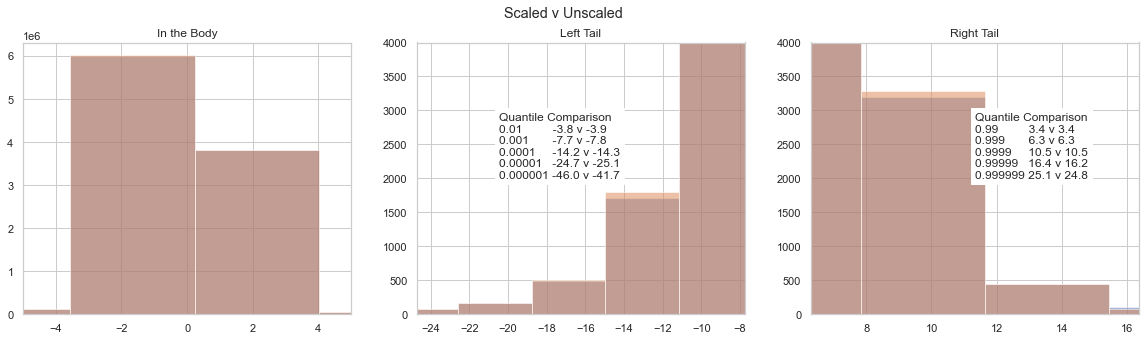
We can confirm this with the Anderson-Darliing test for k-samples from scipy. The null hypothesis is that the two samples come from the same distribution.

[14]:

import scipy.stats as scist

import warnings

with warnings.catch_warnings():
    warnings.simplefilter("ignore", category=UserWarning)

    phats_ad = scist.anderson_ksamp((
        rv1*10,
        rv2
    ))
phats_ad

[14]:

Anderson_ksampResult(statistic=2350120.560339984, critical_values=array([0.325, 1.226, 1.961, 2.718, 3.752, 4.592, 6.546]), significance_level=0.001)

Per the result, we cannot reject that the two samples come from the same distribution. Thus, for convenience going forward, we will scale the PhatNet mu and std parameter outputs by 10.

Comparing Fit¶

We will compare the fit of the residuals to the Phat distribution with that of the Normal by first assessing quantiles.

[15]:

phat = ph.Phat(mu*10, std*10, l, r)

norm_params = scist.norm.fit(garch_resids.flatten())
normfit = scist.norm(*norm_params)

l_crit = 1/np.logspace(2,5,4)
r_crit = 1 - l_crit

l_act = np.quantile(garch_resids.flatten(), l_crit)
nl_act = [(garch_resids.flatten() < q).sum() for q in l_act]

df_lcrit = pd.DataFrame([
    nl_act,
    l_act,
    phat.ppf(l_crit),
    normfit.ppf(l_crit),
], index=['# Obs', 'Actual', 'Phat', 'Gaussian'], columns=l_crit).T

r_act = np.quantile(garch_resids.flatten(), r_crit)
nr_act = [(garch_resids.flatten() > q).sum() for q in r_act]
df_rcrit = pd.DataFrame([
    nr_act,
    r_act,
    phat.ppf(r_crit),
    normfit.ppf(r_crit),
], index=['# Obs', 'Actual', 'Phat', 'Gaussian'], columns=r_crit).T

df_crit = pd.concat((df_lcrit[::-1], df_rcrit))

df_crit

[15]:

	# Obs	Actual	Phat	Gaussian
0.00001	1.0	-10.697492	-25.081239	-4.298209
0.00010	2.0	-8.708911	-14.297968	-3.752568
0.00100	19.0	-4.575658	-7.804973	-3.124053
0.01000	182.0	-2.635801	-3.854028	-2.360494
0.99000	182.0	2.283172	3.385124	2.290214
0.99900	19.0	3.339469	6.280176	3.053772
0.99990	2.0	5.070831	10.412671	3.682287
0.99999	1.0	7.186171	16.377104	4.227928

We can see the quantile values of the actual observations lie somewhere between the Phat and the Normal. The left tail of the Phat also exhibits better fit, to be expected given it has a larger tail index. The difference between the Phat distribution and actual suggests improvements might be made to rein in the Phat distribution somewhat.

We can also check the Anderson-Darling k-sample test for both distributions using draws of standardized random variables.

[16]:

with warnings.catch_warnings():
    warnings.simplefilter("ignore", category=UserWarning)

    norm_ad = scist.anderson_ksamp((
        garch_resids.flatten(),
        normfit.rvs(size=1000000)/normfit.std()
    ))
    phat_ad = scist.anderson_ksamp((
        garch_resids.flatten(),
        phat.std_rvs(size=1000000)
    ))

norm_ad, phat_ad

[16]:

(Anderson_ksampResult(statistic=59.630039694239706, critical_values=array([0.325, 1.226, 1.961, 2.718, 3.752, 4.592, 6.546]), significance_level=0.001),
 Anderson_ksampResult(statistic=119.89759627523853, critical_values=array([0.325, 1.226, 1.961, 2.718, 3.752, 4.592, 6.546]), significance_level=0.001))

We cannot reject the null for either distribution (that it is the true distribution), but the Phat does have a larger statistic.

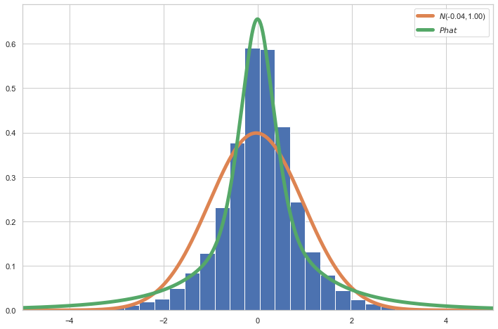
Consistent with the quantile comparison earlier, the Phat performs better than the Gaussian over the head and tail, but underperforms with respecect to the shoulder.

Phatcast¶

Now we have enough to generate an ARMA-GARCH forecast with Phat residuals. We will compare the forecast to the standard Gaussian residuals visually.

[18]:

n = 10000
days = 252

mod = ph.Garchcaster(
    arma=arma22,
    garch=arch11,
    iters=n,
    periods=days,
)
res1 = mod.forecast(dist=phat)
res2 = mod.forecast()

Below, we compare on a 1-year time horizon (252 days).

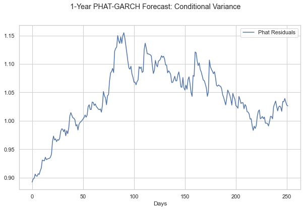
Obviously, for the long-term forecasts, the Phat distribution creates a much more “natural” volatility with short, dramatic spikes, whole periods of elevated levels of volatility, and prolonged periods of sustained, declining and low volatility.

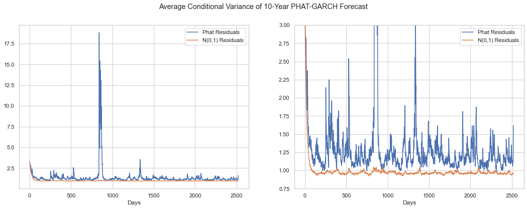
Now, we compare over a 10-year horizon. We show the full spectrum on the left-hand side, then zoom in on the right to show the difference in volatility day-to-day.

[20]:

res3 = mod.forecast(dist=phat, periods=days*10)
res4 = mod.forecast(periods=days*10)

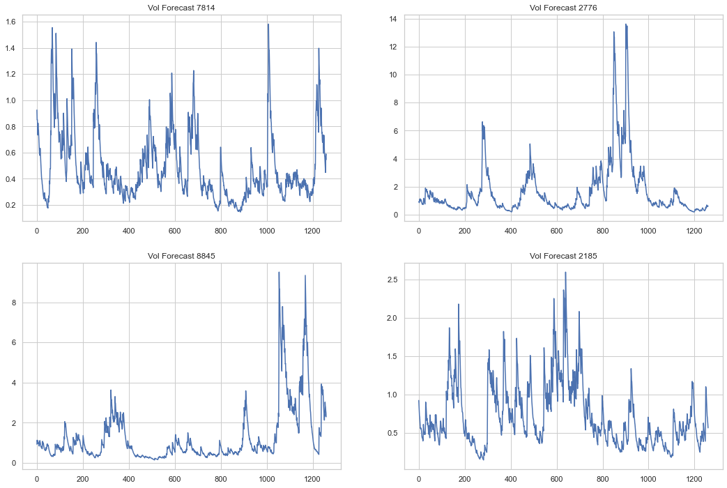
Bear in mind, these are averages across 10,000 simulations. We can show the individual volatilities from each simulations as follows:

[22]:

fig, axs = plt.subplots(2,2,figsize=(18,12))
axs = axs.flatten()

for i, ax in zip(np.random.randint(0, n, size=axs.size), axs):
    ax.plot(res3.vols[i], label='Phat Residuals')
    ax.set_title(f'Vol Forecast {i}')

plt.show()

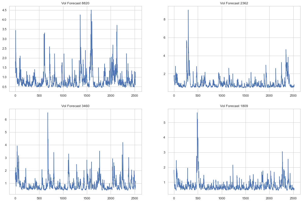
We can see from these samples that a more “natural” volatility process continues for many periods, well after the standard Gaussian has found a stable range. We can compare these volatility outcomes to the actual conditional volatility found the S&P500 time-series below.

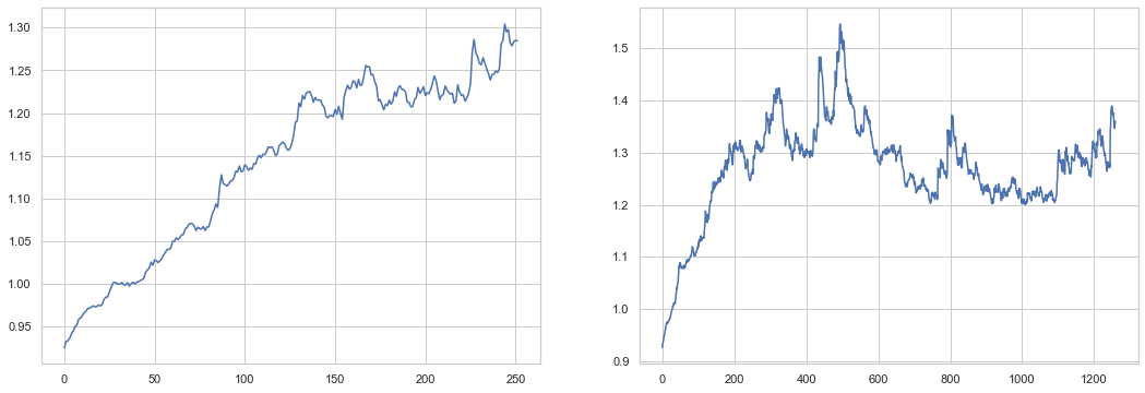
[23]:

fig, (ax1, ax2) = plt.subplots(1,2,figsize=(18,6))

ax1.plot(arch11.conditional_volatility)

ax2.plot(arch11.conditional_volatility)
ax2.set_ylim(0,4)

plt.suptitle('10-Year Actual Historical GARCH-Fitted Conditional Volatility')
plt.show()

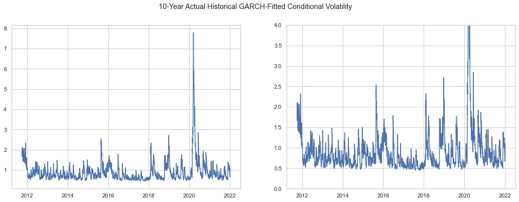
The volatility spikes generated by the Phat distribution may seem dramatic but relative to the spikes seen in 2020 and 2008, they may even be conservative. Note that the Phat residuals are able to mimic the tendency for volatility to stabilize below 1x for significant stretches.

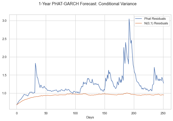
We can replicate this outcome in arch as a test. NOTE this does not include the ARMA process.

[24]:

def custom_rng(phat):
    def _rng(size):
        shocks = phat.std_rvs(size=size)
        return shocks
    return _rng

[25]:

sim1 = arch11.forecast(
    horizon=days,
    simulations=n,
    rng=custom_rng(phat),
    method='simulation',
    reindex=False
)

sim2 = arch11.forecast(
    horizon=days,
    simulations=n,
    method='simulation',
    reindex=False
)

[26]:

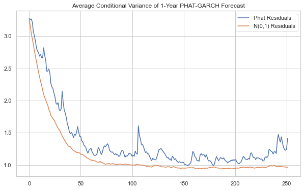
fig, ax1 = plt.subplots(1,1,figsize=(10,6))

ax1.plot(sim1.variance.values.T, label='Phat Residuals')
ax1.plot(sim2.variance.values.T, label='N(0,1) Residuals')

ax1.set_xlabel('Days')
ax1.legend()

plt.suptitle('1-Year PHAT-GARCH Forecast: Conditional Variance')
plt.show()

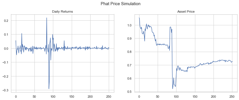
1-Year Price Forecast¶

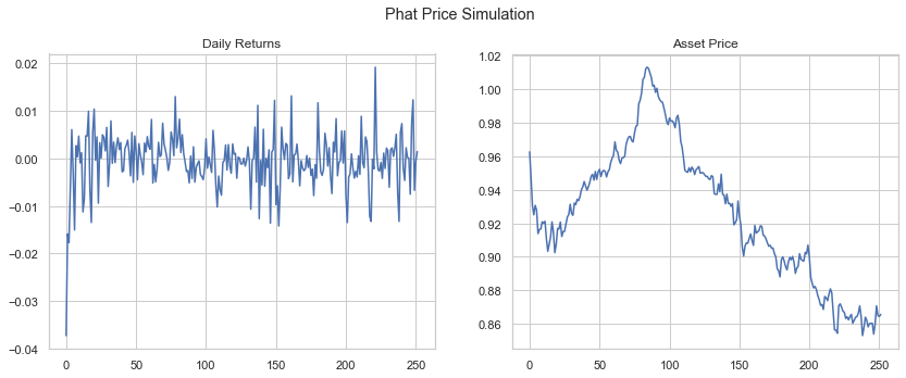
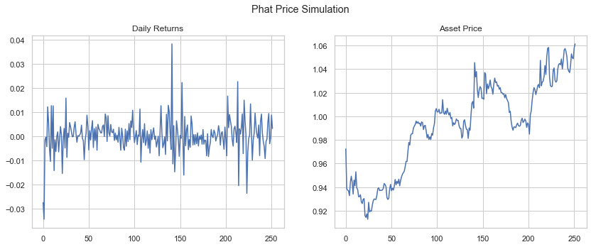
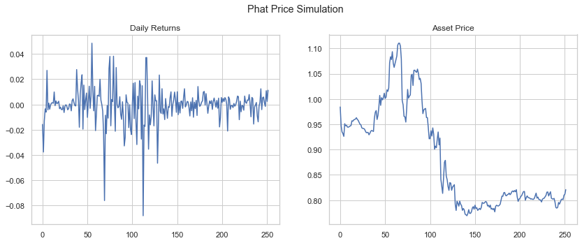
We can generate price forecasts simply by calling the plot method on our GarchcasterResults containers. First, we show 4 sample simulations, assuming a starting price of $1.

[27]:

axes = res1.plot('price', p=1, n=4)

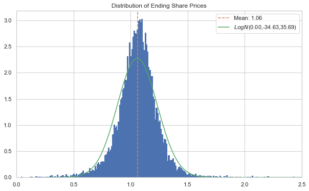
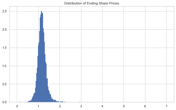
Below we show the end price distribution.

[28]:

ax, S, bins = res1.plot('end_price', p=1)
plt.rcParams['patch.edgecolor'] = 'C0'
ax.axvline(S[:, -1].mean(), c='C1', ls='--', label=f'Mean: {S[:, -1].mean():.2f}')


logps = scist.lognorm.fit(S[:, -1])
x = np.linspace(0, 3.50, 1000)
lnormfit = scist.lognorm.pdf(x, *logps)
ax.plot(x, lnormfit, c='C2', label=r'$LogN$'+f'({logps[0]:.2f},{logps[1]:.2f},{logps[2]:.2f})')

ax.set_xlim(0,4.00)

ax.legend()
plt.show()

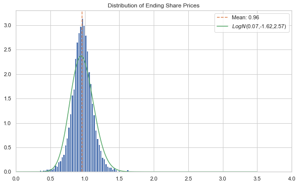
Note three things from above:

The right tail has much higher values than the Gaussian residual forecast; they simply aren’t visible
Because of the much thicker tails, the lognormal fit is completely meaningless. The lognormal simply cannot replicate the distribution appropriately.
Despite having much higher values in the tails, the mean of this distribution is actually lower than the Guassian residual forecast.

Now, again, comparing quantiles, we see the impact of Phat tail volatility on the extremes. The extreme quantiles are much more power-law like.

[29]:

l_crit = 1/np.logspace(1,5,5)
r_crit = 1 - l_crit
qs = np.concatenate((l_crit[::-1], r_crit))
logqs = scist.lognorm(*logps).ppf(qs)

actual = np.quantile(S[:,-1][S[:,-1]>=0], qs)
pd.DataFrame(list(zip(logqs, actual)), index=qs, columns=['Lognorm', 'PHAT-GARCH'])

[29]:

	Lognorm	PHAT-GARCH
0.00001	0.329353	0.014284
0.00010	0.400225	0.055723
0.00100	0.485067	0.218195
0.01000	0.592957	0.533168
0.10000	0.749553	0.782968
0.90000	1.182379	1.142146
0.99000	1.380771	1.388429
0.99900	1.534670	2.106316
0.99990	1.667264	4.524516
0.99999	1.786892	5.912525

Here we see the tail regions of a 1-year price forecast are dramatically larger and likely more realistic.

a ~50% decline is expected about once every hundred years, which maps fairly well onto the S&P 500, which has seen just one annual period of >50% declines since 1950 (and two others fairly close).
a decline of ~87% is expected once every 1,000 years, which has not happened in the history of the S&P, although of course the index did lose ~90% of its value over a three-year period during the Great Depression. Under Guassian innovations, this is essentially impossible.

Phat-ARGARCH¶

In an effort to show the whole process in a more condensed fashion, we will fit and forecast using the arch packages internal AR-GARCH fitting model, which should provide more efficient and accurate fit for both AR and GARCH parameters, though it might ignore some mean correlation.

[27]:

ar = arch.univariate.ARX(sp_ret, lags=[1,2])
ar.volatility = arch.univariate.GARCH(p=1, q=1)
argarch = ar.fit(update_freq=0, disp="off")
print(argarch.summary())

                           AR - GARCH Model Results
==============================================================================
Dep. Variable:                  Close   R-squared:                      -0.007
Mean Model:                        AR   Adj. R-squared:                 -0.007
Vol Model:                      GARCH   Log-Likelihood:               -21745.6
Distribution:                  Normal   AIC:                           43503.1
Method:            Maximum Likelihood   BIC:                           43549.9
                                        No. Observations:                18107
Date:                Sun, Jan 09 2022   Df Residuals:                    18104
Time:                        11:44:48   Df Model:                            3
                                  Mean Model
==============================================================================
                 coef    std err          t      P>|t|        95.0% Conf. Int.
------------------------------------------------------------------------------
Const          0.0506  6.068e-03      8.340  7.408e-17   [3.872e-02,6.251e-02]
Close[1]       0.0801  8.350e-03      9.598  8.160e-22   [6.378e-02,9.651e-02]
Close[2]      -0.0210  8.255e-03     -2.549  1.081e-02 [-3.722e-02,-4.859e-03]
                              Volatility Model
============================================================================
                 coef    std err          t      P>|t|      95.0% Conf. Int.
----------------------------------------------------------------------------
omega          0.0114  2.144e-03      5.316  1.058e-07 [7.197e-03,1.560e-02]
alpha[1]       0.0941  1.071e-02      8.783  1.597e-18   [7.307e-02,  0.115]
beta[1]        0.8956  1.114e-02     80.425      0.000     [  0.874,  0.917]
============================================================================

Covariance estimator: robust

[28]:

data = ph.DataSplit(argarch.std_resid.values[2:]/10)
xil, xir = ph.two_tailed_hill_double_bootstrap(data.raw.y)

[29]:

nnet = ph.PhatNet(neurons=1)

optimizer = tf.keras.optimizers.Adam(learning_rate=5e-4)
nnet.compile(loss=ph.PhatLoss(xil, xir), optimizer=optimizer)
history = nnet.fit(
    data.train,
    epochs=100,
    validation_data=data.test,
    verbose=0
)

Epoch 00015: early stopping

We show a 1-year forecast.

[30]:

mu, std, l, r = nnet.predicted_params().values[:, 0]
phat = ph.Phat(mu, std, l, r)

n = 10000
days = 252

mod = ph.Garchcaster(
    garch=argarch,
    iters=n,
    periods=days,
)
arres = mod.forecast(dist=phat)

[32]:

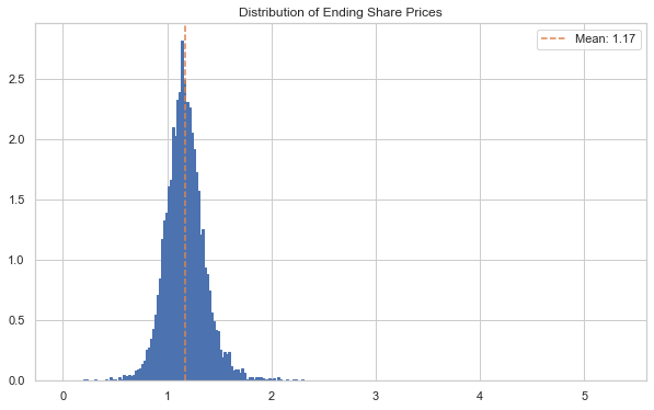
ax, S_phat, bins = arres.plot('end_price', p=1)

ax.axvline(S_phat[:, -1].mean(), c='C1', ls='--', label=f'Mean: {S_phat[:, -1].mean():.2f}')

logps = scist.lognorm.fit(S_phat[:, -1][S_phat[:,-1]>=0])
x = np.linspace(.25, 4, 1000)
lnormfit = scist.lognorm.pdf(x, *logps)
ax.plot(x, lnormfit, c='C2', label=r'$LogN$'+f'({logps[0]:.2f},{logps[1]:.2f},{logps[2]:.2f})')
ax.set_xlim((0,2.5))

ax.legend()
plt.show()

plt.show()

[33]:

l_crit = 1/np.logspace(1,5,5)
r_crit = 1 - l_crit
qs = np.concatenate((l_crit[::-1], r_crit))
logqs = scist.lognorm(*logps).ppf(qs)

arres_actual = np.quantile(S_phat[:,-1][S_phat[:,-1]>=0], qs)
pd.DataFrame(list(zip(logqs, arres_actual)), index=qs, columns=['Lognorm', 'PHAT-GARCH'])

[33]:

	Lognorm	PHAT-GARCH
0.00001	0.317898	0.048463
0.00010	0.411891	0.121818
0.00100	0.520475	0.248225
0.01000	0.652841	0.564735
0.10000	0.834691	0.859879
0.90000	1.284786	1.254197
0.99000	1.469893	1.497912
0.99900	1.605834	1.956817
0.99990	1.718117	2.203955
0.99999	1.815877	2.408279

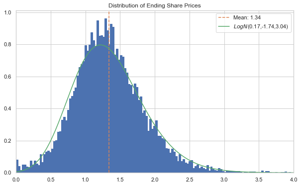
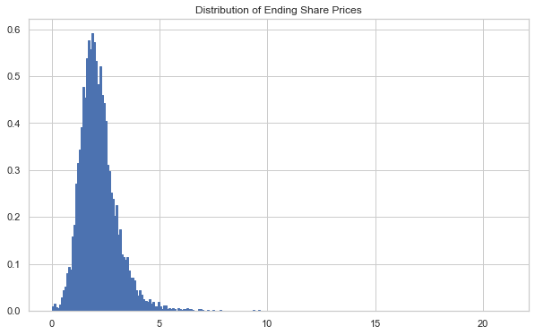
And a 5-year forecast.

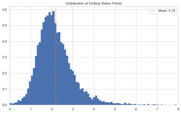
[34]:

arres5 = mod.forecast(dist=phat, periods=252*5)

[35]:

ax, S_5, bins = arres5.plot('end_price', p=1)

ax.axvline(S_5[:, -1].mean(), c='C1', ls='--', label=f'Mean: {S_5[:, -1].mean():.2f}')

logps = scist.lognorm.fit(S_5[:, -1][S_5[:,-1]>=0])
x = np.linspace(0, 10, 1000)
lnormfit = scist.lognorm.pdf(x, *logps)
ax.plot(x, lnormfit, c='C2', label=r'$LogN$'+f'({logps[0]:.2f},{logps[1]:.2f},{logps[2]:.2f})')

ax.set_xlim(0,4)
ax.legend()
plt.show()

plt.show()

[36]:

l_crit = 1/np.logspace(1,5,5)
r_crit = 1 - l_crit
qs = np.concatenate((l_crit[::-1], r_crit))
logqs = scist.lognorm(*logps).ppf(qs)

S5_actual = np.quantile(S_5[:,-1][S_5[:,-1]>=0], qs)
pd.DataFrame(list(zip(logqs, S5_actual)), index=qs, columns=['Lognorm', 'PHAT-ARGARCH'])

[36]:

	Lognorm	PHAT-ARGARCH
0.00001	-0.249066	1.064057e-08
0.00010	-0.106708	1.015339e-07
0.00100	0.074192	2.259743e-03
0.01000	0.321116	2.107520e-01
0.10000	0.714136	7.466369e-01
0.90000	2.025579	1.986490e+00
0.99000	2.743530	2.842280e+00
0.99900	3.353665	4.548018e+00
0.99990	3.917705	5.699216e+00
0.99999	4.457776	6.904041e+00

Pay close attention to the bulge in values around $0. The Phat-ARGARCH suggests that total loss is materially more likely than with Gaussian innvoations.

T v Phat-ARGARCH¶

We will compare the Phat-ARGARCH results to an AR-GARCH fit using the Student’s T.

[37]:

targarch = arch.univariate.ARX(sp_ret, lags=[1,2])
targarch.distribution = arch.univariate.StudentsT()

targarch.volatility = arch.univariate.GARCH(p=1, q=1)
tres = targarch.fit(update_freq=0, disp="off")
print(tres.summary())

                              AR - GARCH Model Results
====================================================================================
Dep. Variable:                        Close   R-squared:                      -0.006
Mean Model:                              AR   Adj. R-squared:                 -0.006
Vol Model:                            GARCH   Log-Likelihood:               -21229.6
Distribution:      Standardized Student's t   AIC:                           42473.3
Method:                  Maximum Likelihood   BIC:                           42527.9
                                              No. Observations:                18107
Date:                      Sun, Jan 09 2022   Df Residuals:                    18104
Time:                              11:45:35   Df Model:                            3
                                  Mean Model
==============================================================================
                 coef    std err          t      P>|t|        95.0% Conf. Int.
------------------------------------------------------------------------------
Const          0.0589  5.014e-03     11.742  7.803e-32   [4.905e-02,6.871e-02]
Close[1]       0.0761  7.661e-03      9.930  3.072e-23   [6.106e-02,9.109e-02]
Close[2]      -0.0327  7.594e-03     -4.301  1.703e-05 [-4.754e-02,-1.777e-02]
                              Volatility Model
============================================================================
                 coef    std err          t      P>|t|      95.0% Conf. Int.
----------------------------------------------------------------------------
omega      8.1892e-03  1.223e-03      6.694  2.168e-11 [5.792e-03,1.059e-02]
alpha[1]       0.0894  6.379e-03     14.019  1.196e-44   [7.693e-02,  0.102]
beta[1]        0.9046  6.533e-03    138.475      0.000     [  0.892,  0.917]
                              Distribution
========================================================================
                 coef    std err          t      P>|t|  95.0% Conf. Int.
------------------------------------------------------------------------
nu             6.4736      0.331     19.538  5.176e-85 [  5.824,  7.123]
========================================================================

Covariance estimator: robust

[38]:

n = 10000
days = 252
mod = ph.Garchcaster(
    garch=tres,
    iters=n,
    periods=days,
)

We can incorporate the fitted T distribution into Garchcast simply by generating standardized random variables from it and passing them to innovs. We will do this for both 1-year and 5-year periods.

[39]:

t_dist = scist.t(tres.params[-1])
tfore1 = mod.forecast(innovs=t_dist.rvs((n, days))/t_dist.std())
tfore2 = mod.forecast(innovs=t_dist.rvs((n, days*5))/t_dist.std(), periods=days*5)

The variance is given below.

[40]:

fig, (ax1, ax2) = plt.subplots(1,2,figsize=(18,6))
ax1 = tfore1.plot('var', ax=ax1)
ax2 = tfore2.plot('var', ax=ax2)

plt.suptitle('T-GARCH Forecast: Conditional Variance')
plt.show()

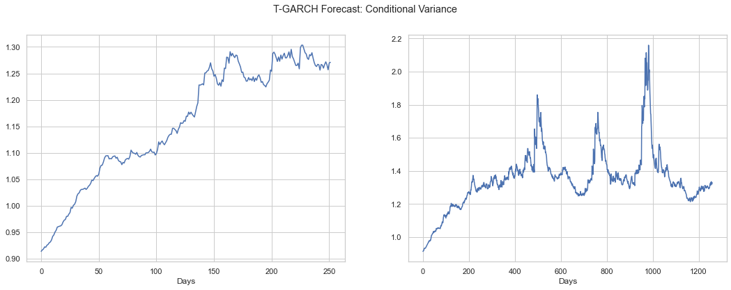
The variance takes more than a year to climb to a stable range, then does exhibit some more “natural” variation around that stable value, although we do not see a single peak, $\sigma^2 > 1.6$ over the course of ten years.

The S&P 500, of course, exhibited several such peaks in the just the past 15 years and the Phat distribution is able to produce them while the T is not.

[41]:

ax, S_t, bins = tfore1.plot('end_price', p=1)

ax.axvline(S_t[:, -1].mean(), c='C1', ls='--', label=f'Mean: {S_t[:, -1].mean():.2f}')

ax.legend()
plt.show()

[42]:

l_crit = 1/np.logspace(1,5,5)
r_crit = 1 - l_crit
qs = np.concatenate((l_crit[::-1], r_crit))
logqs = scist.lognorm(*logps).ppf(qs)

St_actual = np.quantile(S_t[:,-1], qs)
pd.DataFrame(list(zip(St_actual, arres_actual)), index=qs, columns=['T-GARCH', 'PHAT-ARGARCH'])

[42]:

	T-GARCH	PHAT-ARGARCH
0.00001	0.010219	0.048463
0.00010	0.033864	0.121818
0.00100	0.311191	0.248225
0.01000	0.700952	0.564735
0.10000	0.945853	0.859879
0.90000	1.396236	1.254197
0.99000	1.730817	1.497912
0.99900	2.309870	1.956817
0.99990	4.158293	2.203955
0.99999	5.214342	2.408279

[43]:

ax, S_t5, bins = tfore2.plot('end_price', p=1)

ax.axvline(S_t5[:, -1].mean(), c='C1', ls='--', label=f'Mean: {S_t5[:, -1].mean():.2f}')

ax.set_xlim(0, 8)

ax.legend()
plt.show()

[44]:

l_crit = 1/np.logspace(1,5,5)
r_crit = 1 - l_crit
qs = np.concatenate((l_crit[::-1], r_crit))
logqs = scist.lognorm(*logps).ppf(qs)

St5_actual = np.quantile(S_t5[:,-1], qs)
pd.DataFrame(list(zip(St5_actual, S5_actual)), index=qs, columns=['T-GARCH', 'PHAT-ARGARCH'])

[44]:

	T-GARCH	PHAT-ARGARCH
0.00001	-3.146366e-09	1.064057e-08
0.00010	-3.495613e-13	1.015339e-07
0.00100	6.594357e-02	2.259743e-03
0.01000	5.687693e-01	2.107520e-01
0.10000	1.242332e+00	7.466369e-01
0.90000	3.231544e+00	1.986490e+00
0.99000	5.291559e+00	2.842280e+00
0.99900	8.360764e+00	4.548018e+00
0.99990	1.730612e+01	5.699216e+00
0.99999	2.235512e+01	6.904041e+00

Skew T v Phat-ARGARCH¶

We will compare the Phat-ARGARCH results to an AR-GARCH fit using the Student’s T.

[45]:

skargarch = arch.univariate.ARX(sp_ret, lags=[1,2])
skargarch.distribution = arch.univariate.SkewStudent()

skargarch.volatility = arch.univariate.GARCH(p=1, q=1)
skres = skargarch.fit(update_freq=0, disp="off")
print(skres.summary())

                                 AR - GARCH Model Results
=========================================================================================
Dep. Variable:                             Close   R-squared:                      -0.005
Mean Model:                                   AR   Adj. R-squared:                 -0.006
Vol Model:                                 GARCH   Log-Likelihood:               -21214.4
Distribution:      Standardized Skew Student's t   AIC:                           42444.8
Method:                       Maximum Likelihood   BIC:                           42507.2
                                                   No. Observations:                18107
Date:                           Sun, Jan 09 2022   Df Residuals:                    18104
Time:                                   11:45:51   Df Model:                            3
                                  Mean Model
==============================================================================
                 coef    std err          t      P>|t|        95.0% Conf. Int.
------------------------------------------------------------------------------
Const          0.0505  5.239e-03      9.631  5.925e-22   [4.019e-02,6.073e-02]
Close[1]       0.0713  7.763e-03      9.181  4.289e-20   [5.606e-02,8.649e-02]
Close[2]      -0.0378  7.664e-03     -4.937  7.953e-07 [-5.285e-02,-2.281e-02]
                              Volatility Model
============================================================================
                 coef    std err          t      P>|t|      95.0% Conf. Int.
----------------------------------------------------------------------------
omega      7.8852e-03  1.186e-03      6.649  2.944e-11 [5.561e-03,1.021e-02]
alpha[1]       0.0881  6.227e-03     14.155  1.746e-45   [7.593e-02,  0.100]
beta[1]        0.9058  6.424e-03    140.998      0.000     [  0.893,  0.918]
                                 Distribution
==============================================================================
                 coef    std err          t      P>|t|        95.0% Conf. Int.
------------------------------------------------------------------------------
nu             6.6324      0.344     19.282  7.568e-83       [  5.958,  7.307]
lambda        -0.0568  9.809e-03     -5.796  6.811e-09 [-7.607e-02,-3.762e-02]
==============================================================================

Covariance estimator: robust

Garchcast does not support the Skew-T (mainly because it’s a real pain to implement in python), so we will use arch to forecast as well.

We will do this for both 1-year and 5-year periods.

[46]:

n = 10000
days = 252

skfore1 = tres.forecast(horizon=days, simulations=n, method='simulation', reindex=False)
skfore2 = tres.forecast(horizon=days*5, simulations=n, method='simulation', reindex=False)

The variance is given below.

[47]:

fig, axs = plt.subplots(2,2,figsize=(18,12))
axs = axs.flatten()

for i, ax in zip(np.random.randint(0, n, size=axs.size), axs):
    ax.plot(skfore2.simulations.variances[0][i], label='Phat Residuals')
    ax.set_title(f'Vol Forecast {i}')

plt.show()

[48]:

fig, (ax1, ax2) = plt.subplots(1,2,figsize=(18,6))

ax1.plot(np.arange(days).reshape(-1,1), skfore1.variance.T.values)
ax2.plot(np.arange(days*5).reshape(-1,1), skfore2.variance.T.values)

plt.show()

[49]:

from phat.utils import PriceSim

simmer = PriceSim(p0=1, rets=1 + skfore1.simulations.values[0]/100)
r, S_skew, (ax, bins)= simmer.sims(show_chart=True)

[50]:

l_crit = 1/np.logspace(1,5,5)
r_crit = 1 - l_crit
qs = np.concatenate((l_crit[::-1], r_crit))
logqs = scist.lognorm(*logps).ppf(qs)

Sk_actual = np.quantile(S_skew[:,-1], qs)
pd.DataFrame(list(zip(Sk_actual, arres_actual)), index=qs, columns=['T-GARCH', 'PHAT-ARGARCH'])

[50]:

	T-GARCH	PHAT-ARGARCH
0.00001	0.099531	0.048463
0.00010	0.134222	0.121818
0.00100	0.388800	0.248225
0.01000	0.705946	0.564735
0.10000	0.943368	0.859879
0.90000	1.389228	1.254197
0.99000	1.784811	1.497912
0.99900	2.552943	1.956817
0.99990	4.106211	2.203955
0.99999	6.715764	2.408279

[51]:

simmer = PriceSim(p0=1, rets=1 + skfore2.simulations.values[0]/100)
r, S_skew5, (ax, bins)= simmer.sims(show_chart=True)

[52]:

l_crit = 1/np.logspace(1,5,5)
r_crit = 1 - l_crit
qs = np.concatenate((l_crit[::-1], r_crit))

Ssk5_actual = np.quantile(S_skew5[:,-1], qs)
pd.DataFrame(list(zip(Ssk5_actual, S5_actual)), index=qs, columns=['T-GARCH', 'PHAT-ARGARCH'])

[52]:

	T-GARCH	PHAT-ARGARCH
0.00001	0.001150	1.064057e-08
0.00010	0.001293	1.015339e-07
0.00100	0.110723	2.259743e-03
0.01000	0.563082	2.107520e-01
0.10000	1.219087	7.466369e-01
0.90000	3.241316	1.986490e+00
0.99000	5.311174	2.842280e+00
0.99900	11.537288	4.548018e+00
0.99990	18.693370	5.699216e+00
0.99999	20.831648	6.904041e+00

We can see above that both the T and Skew-T distributions tend to create time-series with fatter right-tails than the Phat distribution, although the Phat is more dramatic in the left. This results due to the large left-tail index found when fitting the Phat distribution.

CAVEATS¶

While GARCH models have been shown to outperform constant volatility models, stochastic volatility has become more popular recently and will be explored at a future date.

phat-tails 0.0.11 documentation

Phat-GARCH¶

Approach¶

A Note on Scaling¶

Forecasting Time Series with Pareto Hybrids¶

Generate ARMA-GARCH Residuals¶

Fit Residuals to the Phat Distribution¶

Some More Notes on Scaling¶

Comparing Fit¶

Phatcast¶

1-Year Price Forecast¶

Phat-ARGARCH¶

T v Phat-ARGARCH¶

Skew T v Phat-ARGARCH¶

CAVEATS¶