.ipynb .pdf

repository open issue suggest edit

Contents

Characteristics

Defining the various characteristics of the CarBen and Phat distributions.

Density

Phat

The Phat distribution density is simply s weighted average of the constituent left and right CarBens.

\[\begin{split}f(x) = \sum\limits_{i=1}^nw_if_i(x) \\f(x) = 0.5*f_{\textit{left}}(x) + 0.5*f_{\textit{right}}(x)\end{split}\]

Right CarBen

The density of the CarBen is a piecewise function as detailed by Carreau and Bengio.

\[\begin{split}f_{\textit{right}}(x) = \left\{ \begin{array}{ll} \frac{1}{\gamma} f_{\mu,\sigma}(x) & \text{if } x\leq a \\ \frac{1}{\gamma} g_{\xi,a,b}(x) & \text{if } x > a\\ \end{array} \right.\end{split}\]

Left CarBen

When reflected to the left-side, we simply flip the valence of the \(x\) and Pareto location, \(a\).

\[\begin{split}f_{\textit{left}}(x) = \left\{ \begin{array}{ll} \frac{1}{\gamma} g_{\xi,-a,b}(-x) & \text{if } x < a \\ \frac{1}{\gamma} f_{\mu,\sigma}(x) & \text{if } x \geq a\\ \end{array} \right.\end{split}\]

Cumulative Distribution Function

Phat

Like the PDF, the Cumulative Distribution Function (CDF) of the Phat distribution is just the weighted average of the component CDFs.

\[\begin{split}F(x) = \sum\limits_{i=1}^nw_iF_i(x) \\f(x) = 0.5*F_{\textit{left}}(x) + 0.5*F_{\textit{right}}(x)\end{split}\]

Right CarBen

The CDF of the CarBen is also piece-wise, expressed as follows for the right.

\[\begin{split}F_{\textit{right}}(x) = \left\{ \begin{array}{ll} \frac{1}{\gamma} F_{\mu,\sigma}(x) & \text{if } x\leq a \\ \frac{1}{\gamma} \left(F_{\mu,\sigma}(a) + G_{\xi,a,b}(x)\right) & \text{if } x > a\\ \end{array} \right.\end{split}\]

Thus, the CDF is simply the sum of the Gaussian and Pareto components.

Left CarBen

The formula for the left CarBen is only slight more complicated. As with the other functions, the CDF of the left CarBen is a summation of its components. The CDF is scaled left-to-right, so in the left instance the first component incorporated is the generalized Pareto. The Pareto tail is a reflected version of its right-tailed cousin, so the CDF of the left is equivalent to the survival function of the right. And we know the reflection is achieved by reversing the valence of \(a\) and \(x\).

\[G_{\textit{left}}(x) = \frac{1}{\gamma}\left(1 - G_{\xi,-a,b}(-x)\right)\]

And this handles the CDF up to the junction \(a\). Equal to and beyond \(a\), we must determine how to sum the CDF of Pareto and the Gaussian. When \(x=a\),

\[1 - G_{\xi,-a,b}(-a) = 1\]

and

\[G_{\textit{left}}(a) = \frac{1}{\gamma}\]

For the Gaussian, we must exclude the left-tail portion and so calculate the CDF on the interval \([a, x)\), which is equivalent to:

\[F_{\mu,\sigma}(x) - F_{\mu,\sigma}(a)\]

This results in:

\[\frac{1}{\gamma}\left(1+ F_{\mu,\sigma}(x) - F_{\mu,\sigma}(a)\right)\]

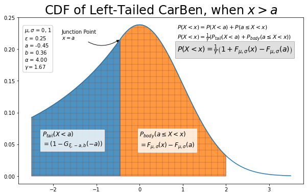
Putting the pieces together results in:

\[\begin{split}F_{\textit{left}}(x) = \left\{ \begin{array}{ll} \frac{1}{\gamma}\left(1 - G_{\xi,-a,b}(-x)\right) & \text{if } x < a \\ \frac{1}{\gamma}\left(1+ F_{\mu,\sigma}(x) - F_{\mu,\sigma}(a)\right) & \text{if } x \geq a\\ \end{array} \right.\end{split}\]

Quantile Function

Phat

Once again, the Quantile Function \(Q(.)\), known in scipy as the percent-point function, ppf, for the Phat distribution is a weighted average of the CarBens.

\[\begin{split}Q(x) = \sum\limits_{i=1}^nw_iQ_i(x) \\Q(x) = 0.5*Q_{\textit{left}}(x) + 0.5*Q_{\textit{right}}(x)\end{split}\]

Right CarBen

Before we derive \(Q(x)\) for each CarBen, it is helpful to know the quantile of the junction point between the tail and body distributions. We know this point to be the location parameter, \(a\), of the generalized Pareto. We also know the relationship between the junction point and \(\gamma\). For the right CarBen,

\[P(X>a) = \frac{1}{\gamma}\]

Quantiles are, of course, merely the cumulative distribtion up to the given point. So the junction quantile, available via the qjunc method, is merely:

\[P(X\leq a) = 1 - P(X>a) = 1 - \frac{1}{\gamma}\]

So, for the right-tailed CarBen, first remember the definition of the Quantile function:

\[x = Q(P(X<x)) = Q(F(x))\]

where, in this framing, we refer to \(P(X\leq x)\) or \(F(x)\) as the quantile. One important difference between the Q derivation and the PDF/CDF derivations above is that the Q function is not a summation of the body and tail Q functions. Q(.) identifies a value derived specifically and solely from the distribution from which it originates. That means, for a right-tailed CarBen,

\[\begin{split}x = \left\{ \begin{array}{ll} Q_{\textit{body}}(P_{\textit{body}}(X<x)) & \text{if } x < a \\ Q_{\textit{tail}}(P_{\textit{tail}}(X<x)) & \text{if } x \geq a\\ \end{array} \right.\end{split}\]

Remember, the input to the Quantile function is a cumulative probability for the entire piecewise, hybrid CarBen. So we must conver that probability, \(P(X<x)\), into \(P_{\textit{body}}(X<x)\) or \(P_{\textit{tail}}(X<x)\) to find the correct value.

So, for all \(x\),

\[P(X<x) = P(X\leq a) + P(a<X<x)\]

Recall:

\[\begin{split}\text{quantile, q} = P(X<x) \\\text{qjunc}, q_a = P(X\leq a) \\P_{tail}(X<a) = 0\end{split}\]

so, where \(x\leq a\),

\[\begin{split}P(X<x) = \frac{P_{\textit{body}}(X<x)}{\gamma} \\P_{\textit{body}}(X<x) = \gamma*P(X<x) = \gamma q\end{split}\]

and where \(x>a\),

\[\begin{split}P(X<x) = q_a + P_{\textit{tail}}(X<x) / \gamma \\P_{\textit{tail}}(X<x) = \gamma(P(X<x) - q_a) = \gamma(q - q_a)\end{split}\]

So, for the right-tail CarBen, the Quantile function for a given \(q = P(X<x)\):

\[\begin{split}x = \left\{ \begin{array}{ll} Q_{\textit{body}}(\gamma q) & \text{if } x \leq a \\ Q_{\textit{tail}}(\gamma q - \gamma q_a) & \text{if } x > a\\ \end{array} \right.\end{split}\]

Left CarBen

As we’ve seen, the left-tailed CarBen requires slight modifications to the formulas. For the qjunc, remember that that CDF of the left-tailed Pareto is equivalent to the Survival Function of the right-tailed, with location, \(a\), reflected so:

\[P_{\textit{right}}(X>a) = \frac{1}{\gamma}\]

\[\text{qjunc } q_a = P_{\textit{left}}(X<a) = P_{\textit{right}}(X>-a) = \frac{1}{\gamma}\]

again available via the qjunc method.

For the Quantile function, we rearrange the piecewise components as follows:

\[\begin{split}x = \left\{ \begin{array}{ll} Q_{\textit{tail}}(P_{\textit{tail}}(X<x)) & \text{if } x < a \\ Q_{\textit{body}}(P_{\textit{body}}(X<x)) & \text{if } x \geq a\\ \end{array} \right.\end{split}\]

We want to express the target left-tailed x value and the Quantile function in terms of the right-tailed x and right Quantile function. This means:

\[\begin{split}P_{\textit{left}}(X<x_{\textit{left}}) = (1 - P_{\textit{right}}(X<x_{\textit{right}})) \\x_{\textit{left}} = -x_{\textit{right}}\end{split}\]

Beginning again with, for all \(x\),

\[P(X<x) = P(X<a) + P(a\leq X<x)\]

so, where \(x<a\),

\[\begin{split}P_{\textit{left}}(X<x_{\textit{left}}) = \frac{P_{\textit{left, tail}}(X<x_{\textit{left}})} {\gamma} \\q = \frac{(1 - P_{\textit{right, tail}}(X<x_{\textit{right, tail}}))} {\gamma} \\P_{\textit{right, tail}}(X<x_{\textit{right, tail}})) = 1 - \gamma q \\x_{\textit{right}} = Q_{\textit{right}}(.) \\Q_{\textit{tail}}(.) = x_{\textit{left}} = -x_{\textit{right}} = -Q_{\textit{right}}(1 - \gamma q)\end{split}\]

And where \(x\geq a\), first, recall in the body,

\[P_{\textit{body}}(a\leq X<x) = P_{\textit{body}}(X<x) - P_{\textit{body}}(X\leq a)\]

We also know that,

\[P_{\textit{body}}(X<a) = 2\gamma q_a - \gamma = \gamma(2q_a-1)\]

So,

\[\begin{split}P_{\textit{left}}(X<x_{\textit{left}}) = q_a + \frac{P_{\textit{body}}(X<x_{\textit{left}})}{\gamma} - \frac{P_{\textit{body}}(X<a)}{\gamma} \\\gamma(q-q_a) = P_{\textit{body}}(X<x_{\textit{left}}) - P_{\textit{body}}(X<a)) \\P_{\textit{body}}(X<x_{\textit{right}}) = \gamma(q-q_a) + P_{\textit{body}}(X<a) \\P_{\textit{body}}(X<x_{\textit{right}}) = \gamma(q-q_a) + \gamma(2q_a-1) \\P_{\textit{body}}(X<x_{\textit{right}}) = \gamma(q-q_a + 2q_a-1) \\P_{\textit{body}}(X<x_{\textit{right}}) = \gamma(q + q_a - 1)\end{split}\]

In the body, realize that \(x_{\textit{left}} = x_{\textit{right}}\)

\[\begin{split}\\x_{\textit{right}} = Q_{\textit{right}}(.) \\Q_{\textit{body}}(.) = x_{\textit{left}} = x_{\textit{right}} = Q_{\textit{body}}(\gamma(q + q_a - 1))\end{split}\]

The end results is:

\[\begin{split}x = \left\{ \begin{array}{ll} -Q_{\textit{right, tail}}(1 - \gamma q) & \text{if } x < a \\ Q_{\textit{body}}(\gamma q + \gamma q_a - \gamma) & \text{if } x \geq a\\ \end{array} \right.\end{split}\]

Moments

Here we show how to find the moments of the Phat distribution. As we know, the Phat distribution is a mixture model of two Carben distributions, each weighted 50%. Thus, the PDF of the Phat distribution is simply:

\[\begin{split}f(x) = \sum\limits_{i=1}^nw_if_i(x) \\f(x) = 0.5*f_{\textit{left}}(x) + 0.5*f_{\textit{right}}(x)\end{split}\]

The Carben distribution has a piecewise density function, defined for a right-tail as:

\[\begin{split}f_{\textit{right}}(x) = \left\{ \begin{array}{ll} \frac{1}{\gamma} f_{\mu,\sigma}(x) & \text{if } y\leq a \\ \frac{1}{\gamma} g_{\xi,a,b}(x) & \text{if } y > a\\ \end{array} \right.\end{split}\]

And for the left

\[\begin{split}f_{\textit{left}}(x) = \left\{ \begin{array}{ll} \frac{1}{\gamma} g_{\xi,-a,b}(-x) & \text{if } y < a \\ \frac{1}{\gamma} f_{\mu,\sigma}(x) & \text{if } y \geq a\\ \end{array} \right.\end{split}\]

The MGF for a mixture model is simply the weighted average of MGF’s of its components, shown as follows:

\[\begin{split}M_x(n) = \int_{-\infty}^{+\infty}e^{nx}f_X(x)\delta x \\ = \int_{-\infty}^{+\infty}e^{nx}\left(.5*f_{\textit{left}}(x) + .5*f_{\textit{right}}(x)\right)\delta x\end{split}\]

\[\begin{split}\\ = \int_{-\infty}^{+\infty}.5*e^{nx}f_{\textit{left}}(x) + .5*e^{nx}f_{\textit{right}}(x)\delta x \\ = .5\int_{-\infty}^{+\infty}e^{nx}f_{\textit{left}}(x)\delta x + .5\int_{-\infty}^{+\infty}e^{nx}f_{\textit{right}}(x)\delta x \\ = .5*M_{left} + .5*M_{right}\end{split}\]

Thus, to find the moments of the Phat, we must find the MGFs of the component Carbens.

Carben Right

The MGF of a piecewise distribution is simply the sum of the integrals along the bounded ranges.

\[M_{right}(n) = \frac{1}{\gamma}\int_{-\infty}^{a}e^{nx}f_{\mu,\sigma}(x)\delta x + \frac{1}{\gamma}\int_{a}^{+\infty}e^{nx}g_{\xi,a,b}(x)\delta x\]

The body term is a truncated normal distribution. The moments of such functions are known and available in scipy. We know that the generalized Pareto is always restricted the interval \((a,\infty)\), so the tail term is merely the MGF of generalized Pareto scaled by \(\frac{1}{\gamma}\). Thus,

\[\frac{1}{\gamma}M_{\mu,\sigma,u}(n) + \frac{1}{\gamma}M_{\xi,a,b}(n)\]

where: \(u\) is the upper bound of the body

Carben Left

Now for the left:

\[\begin{split}M_{left}(n) = \frac{1}{\gamma}\int_{-\infty}^{a}e^{nx}g_{\xi,-a,b}(-x)\delta x + \frac{1}{\gamma}\int_{a}^{+\infty}e^{nx}f_{\mu,\sigma}(x)\delta x \\=\frac{1}{\gamma}\int_{-a}^{+\infty}e^{nx}g_{\xi,-a,b}(x)\delta x + \frac{1}{\gamma}\int_{a}^{+\infty}e^{nx}f_{\mu,\sigma}(x)\delta x\end{split}\]

Once again, the tail portion is the MGF of the generalized Pareto. And once again, the body portion is a truncated normal, this time with a lower bound, so the MGF is found as:

\[\frac{1}{\gamma}M_{\xi,-a,b}(n) + \frac{1}{\gamma}M_{\mu,\sigma,l}(n)\]

where: \(l\) is the lower bound of the body

Mean

The first moment is the first derivative of \(M\), so:

\[\begin{split}\mu_{\textit{right}} = \frac{d}{dx}\frac{1}{\gamma}M_{\mu,\sigma,u}(1) + \frac{d}{dx}\frac{1}{\gamma}M_{\xi,a,b}(1) \\\mu_{\textit{left}} = \frac{d}{dx}\frac{1}{\gamma}M_{\xi,-a,b}(1) + \frac{d}{dx}\frac{1}{\gamma}M_{\mu,\sigma,l}(1)\end{split}\]

In both instances, the constant multiplicative survives the differentiations. For the left tail, in order to reflect its true location, \(a\), we must invert the sign:

\[\begin{split}\mu_{\textit{phat}} = .5*\mu_{\textit{right}} + .5*\mu_{\textit{left}} \\\mu_{\textit{right}} = \frac{1}{\gamma}\text{Mean}_{\mu,\sigma,u} + \frac{1}{\gamma}\text{Mean}_{\xi,a,b} \\\mu_{\textit{left}} = -\frac{1}{\gamma}\text{Mean}_{\xi,-a,b} + \frac{1}{\gamma}\text{Mean}_{\mu,\sigma,l}\end{split}\]

Finding mean of the Phat distribution programmatically is thus fairly trivial.

import numpy as np
import scipy.stats as scist

import phat as ph

phat = ph.Phat(.1, .2, .2, .25)

bmu = scist.truncnorm(
    -np.inf,
    phat.right.a,
    *phat.right.body.args
).mean()
tmu = phat.right.tail.mean()
rmu = (bmu + tmu) / phat.right.gamma

bmu = scist.truncnorm(
    phat.left.a,
    np.inf,
    *phat.left.body.args
).mean()
tmu = -phat.left.tail.mean()
lmu = (bmu + tmu) / phat.left.gamma

The mean of the Phat distribution is:

np.mean((lmu, rmu))

0.1426574558489754

We can see the mean of the Phat in the above example is close to, but slightly higher than the mean of the Gaussian body, \(\mu\). This results from the greater tail index in the right tail used in the example.

phat.mean()

0.1426574558489754

Variance

The second moment is the second derivative of \(M\), so:

\[\begin{split}\text{Var}_{\textit{right}} = \frac{d^2}{dx}\frac{1}{\gamma}M_{\mu,\sigma,u}(2) + \frac{d^2}{dx}\frac{1}{\gamma}M_{\xi,a,b}(2) \\\text{Var}_{\textit{left}} = \frac{d^2}{dx}\frac{1}{\gamma}M_{\xi,-a,b}(2) + \frac{d^2}{dx}\frac{1}{\gamma}M_{\mu,\sigma,l}(2) \\\text{Var}_{\textit{right}} = \frac{1}{\gamma}\text{Var}_{\mu,\sigma,u} + \frac{1}{\gamma}\text{Var}_{\xi,a,b} \\\text{Var}_{\textit{left}} = \frac{1}{\gamma}\text{Var}_{\xi,-a,b} + \frac{1}{\gamma}\text{Var}_{\mu,\sigma,l} \\\text{Var}_{\textit{phat}} = .5*\text{Var}_{\textit{right}} + .5*\text{Var}_{\textit{left}}\end{split}\]

Note that no negative is applied to the second moment as it eliminated bystanders the square.

And so the variance of the Phat is found as:

bvar = scist.truncnorm(
    -np.inf,
    phat.right.a,
    *phat.right.body.args
).var()
tvar = phat.right.tail.var()
rvar = (bvar + tvar) / phat.right.gamma

bvar = scist.truncnorm(
    phat.left.a,
    np.inf,
    *phat.left.body.args
).var()
tvar = phat.left.tail.var()
lvar = (bvar + tvar) / phat.left.gamma

lvar

0.4828404012432034

The variance for the Phat distribution is then:

np.mean((lvar, rvar))

0.5732923559721449

This is available as var method of the Phat distribution.

phat.var()

0.5732923559721449

the Phat Distribution Peak-Over Threshold