Here we explore methods for financial time-series forecasts that incorporate Gaussian models. We outline tools in the phat package that can be used to simulate such time-series.
ARMA-GARCH for Time Series
Up to now we have assumed that each daily draw from a financial time-series is both independent and stationary. This is likely not the case.
There is much debate as to exactly how, but it is more likely that return time series are both correlated to near-term historical returns and trend over various timeframes. For example, Mandelbrot’s MultiFractal Model incorporates a form of “long memory”.
Here, we will familiarize ourselves with the ARMA models accounting for correlation in the mean and GARCH models accounting for correlation in the volatility. Later on, we will incorporate the Phat distribution into these models.
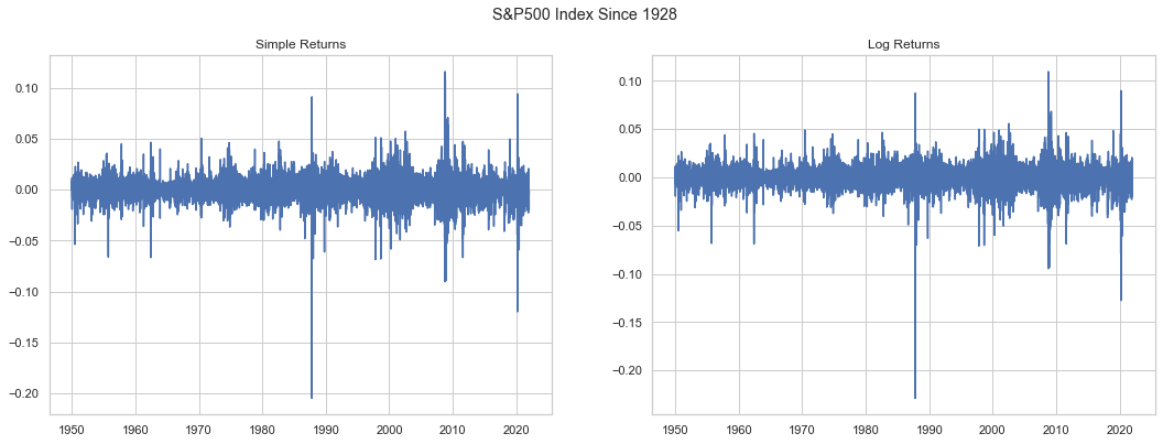
First, we download the full S&P500 daily time series from YAHOO!.
Then we find both the simple and log returns. There is much debate in finance regarding “simple v log” returns (Hudson and Gregoriou (2013)). Most arguments in favor of log returns tend to focus on their Gaussian properties. Of course, the Gaussian distribution, and attempts to squeeze the world into it, are anathema to the study of fat tails.
It is common to use log returns in ARMA-GARCH models (Barigozzi(2014)), however, they have some limiting statistical properties and can lead to a very different mean/volatility structure.
We will explore the utilization of both going forward. Note the ^GSPC time series recently reduced to weekly data points for most the 1940s. So we will start the analysis beginning with 1950.
[86]:
import numpy as np
import yfinance as yf

sp = yf.download('^GSPC')
sp_ret = sp.Close.pct_change().loc['1950-01-01':]
sp_lret = np.log1p(sp.Close.pct_change()).loc['1950-01-01':]
[*********************100%***********************] 1 of 1 completed
Non-Stationarity
Stationarity is a key requirement of ARMA models. In time series, non-stationarity is usually evidenced by some trend, either via drift from the process itself or a deterministic component of time.
The augmented Dickey-Fuller test can be used to detect non-stationarity. The null hypothesis is non-stationary, so if the test statistic is lower than the threshold statistic, non-stationarity can be rejected.
First, we will test daily prices.
[88]:
from statsmodels.tsa.stattools import adfuller

adf, p_value, _, _, crit, _ = adfuller(sp.Close, regression='ct')
adf, crit['10%']
[88]:
(4.466060325077834, -3.1271811390158364)
So, daily S&P500 prices appear to be non-stationary. Now, we will test both simple and log returns.
[89]:
adf, p_value, _, _, crit, _ = adfuller(sp_lret*100, regression='ct')
adf, crit['1%'], p_value
[89]:
(-23.524567833117075, -3.9592709501073697, 0.0)
[90]:
adf, p_value, _, _, crit, _ = adfuller(sp_ret*100, regression='ct')
adf, crit['1%'], p_value
[90]:
(-23.781397137877068, -3.9592709501073697, 0.0)
The outcome is the complete opposite. The test statistic is well below the 1% threshold and the p-value is zero. The outcome also seems independent of the log return discussion.
Here we see the value in utilizing returns for financial time-series.
ARMA
There are two approaches to formulating ARMA-GARCH models. The first is a two-step process that fits the mean process first (ARMA) and then applies GARCH to the residuals. The second fits both the mean and volatility processes simultaneously.
For ARMA-fitting, there are two packages: statsmodels and pmdarima, with the latter being favored as it has an auto_arima function that finds the best model automatically.
For GARCH, the arch model is used. arch has the ability to AR-GARCH simultaneously. Moving Average (MA) models must be fit to the residuals.
We will demonstrate the two-step process. First, fit the ARMA via pmdarima for both simple and log returns.
[91]:
import pmdarima

sparmasim = pmdarima.auto_arima(sp_ret)
sparmasim.summary()
[91]:
| Dep. Variable: | y | No. Observations: | 18109 |
|---|---|---|---|
| Model: | SARIMAX | Log Likelihood | 57956.613 |
| Date: | Sun, 09 Jan 2022 | AIC | -115909.227 |
| Time: | 09:30:11 | BIC | -115893.619 |
| Sample: | 0 | HQIC | -115904.096 |
| - 18109 | |||
| Covariance Type: | opg |
| coef | std err | z | P>|z| | [0.025 | 0.975] | |
|---|---|---|---|---|---|---|
| intercept | 0.0004 | 7.39e-05 | 4.872 | 0.000 | 0.000 | 0.001 |
| sigma2 | 9.72e-05 | 3.03e-07 | 320.893 | 0.000 | 9.66e-05 | 9.78e-05 |
| Ljung-Box (L1) (Q): | 0.05 | Jarque-Bera (JB): | 339526.20 |
|---|---|---|---|
| Prob(Q): | 0.83 | Prob(JB): | 0.00 |
| Heteroskedasticity (H): | 3.03 | Skew: | -0.65 |
| Prob(H) (two-sided): | 0.00 | Kurtosis: | 24.17 |
Warnings:
[1] Covariance matrix calculated using the outer product of gradients (complex-step).
[92]:
sparmalog = pmdarima.auto_arima(sp_lret)
sparmalog.summary()
[92]:
| Dep. Variable: | y | No. Observations: | 18109 |
|---|---|---|---|
| Model: | SARIMAX | Log Likelihood | 57883.879 |
| Date: | Sun, 09 Jan 2022 | AIC | -115763.758 |
| Time: | 09:30:20 | BIC | -115748.149 |
| Sample: | 0 | HQIC | -115758.626 |
| - 18109 | |||
| Covariance Type: | opg |
| coef | std err | z | P>|z| | [0.025 | 0.975] | |
|---|---|---|---|---|---|---|
| intercept | 0.0003 | 7.5e-05 | 4.154 | 0.000 | 0.000 | 0.000 |
| sigma2 | 9.798e-05 | 2.76e-07 | 354.629 | 0.000 | 9.74e-05 | 9.85e-05 |
| Ljung-Box (L1) (Q): | 0.01 | Jarque-Bera (JB): | 546895.46 |
|---|---|---|---|
| Prob(Q): | 0.91 | Prob(JB): | 0.00 |
| Heteroskedasticity (H): | 3.03 | Skew: | -1.03 |
| Prob(H) (two-sided): | 0.00 | Kurtosis: | 29.84 |
Warnings:
[1] Covariance matrix calculated using the outer product of gradients (complex-step).
So, we have a strange result here. Both the simple and the log returns return a constant!
Importance of Scale
We will see here and later on the importance of appropriate scale for ARMA and GARCH fitting. Share price returns have very small differences that impact the weighting of likelihood models. As a result, returns are often scaled by 100 (showing in percentage terms).
[93]:
sparmasim100 = pmdarima.auto_arima(sp_ret*100)
sparmasim100.summary()
[93]:
| Dep. Variable: | y | No. Observations: | 18109 |
|---|---|---|---|
| Model: | SARIMAX(2, 0, 2) | Log Likelihood | -25428.936 |
| Date: | Sun, 09 Jan 2022 | AIC | 50869.872 |
| Time: | 09:31:29 | BIC | 50916.697 |
| Sample: | 0 | HQIC | 50885.266 |
| - 18109 | |||
| Covariance Type: | opg |
| coef | std err | z | P>|z| | [0.025 | 0.975] | |
|---|---|---|---|---|---|---|
| intercept | 0.0136 | 0.005 | 2.859 | 0.004 | 0.004 | 0.023 |
| ar.L1 | 0.0512 | 0.070 | 0.728 | 0.467 | -0.087 | 0.189 |
| ar.L2 | 0.5714 | 0.066 | 8.669 | 0.000 | 0.442 | 0.701 |
| ma.L1 | -0.0527 | 0.069 | -0.763 | 0.445 | -0.188 | 0.083 |
| ma.L2 | -0.5976 | 0.065 | -9.211 | 0.000 | -0.725 | -0.470 |
| sigma2 | 0.9710 | 0.003 | 306.783 | 0.000 | 0.965 | 0.977 |
| Ljung-Box (L1) (Q): | 0.00 | Jarque-Bera (JB): | 337167.61 |
|---|---|---|---|
| Prob(Q): | 0.97 | Prob(JB): | 0.00 |
| Heteroskedasticity (H): | 3.02 | Skew: | -0.73 |
| Prob(H) (two-sided): | 0.00 | Kurtosis: | 24.09 |
Warnings:
[1] Covariance matrix calculated using the outer product of gradients (complex-step).
[94]:
sparmalog100 = pmdarima.auto_arima(sp_lret*100)
sparmalog100.summary()
[94]:
| Dep. Variable: | y | No. Observations: | 18109 |
|---|---|---|---|
| Model: | SARIMAX(4, 0, 4) | Log Likelihood | -25483.385 |
| Date: | Sun, 09 Jan 2022 | AIC | 50986.769 |
| Time: | 09:36:36 | BIC | 51064.811 |
| Sample: | 0 | HQIC | 51012.426 |
| - 18109 | |||
| Covariance Type: | opg |
| coef | std err | z | P>|z| | [0.025 | 0.975] | |
|---|---|---|---|---|---|---|
| intercept | 0.0173 | 0.005 | 3.655 | 0.000 | 0.008 | 0.027 |
| ar.L1 | -0.1248 | 0.056 | -2.237 | 0.025 | -0.234 | -0.015 |
| ar.L2 | 1.3699 | 0.060 | 22.886 | 0.000 | 1.253 | 1.487 |
| ar.L3 | -0.0073 | 0.046 | -0.158 | 0.875 | -0.097 | 0.083 |
| ar.L4 | -0.7844 | 0.046 | -17.076 | 0.000 | -0.874 | -0.694 |
| ma.L1 | 0.1312 | 0.056 | 2.330 | 0.020 | 0.021 | 0.241 |
| ma.L2 | -1.3937 | 0.060 | -23.058 | 0.000 | -1.512 | -1.275 |
| ma.L3 | -0.0005 | 0.047 | -0.010 | 0.992 | -0.093 | 0.092 |
| ma.L4 | 0.7903 | 0.047 | 16.692 | 0.000 | 0.698 | 0.883 |
| sigma2 | 0.9777 | 0.003 | 323.204 | 0.000 | 0.972 | 0.984 |
| Ljung-Box (L1) (Q): | 0.61 | Jarque-Bera (JB): | 532266.89 |
|---|---|---|---|
| Prob(Q): | 0.43 | Prob(JB): | 0.00 |
| Heteroskedasticity (H): | 3.02 | Skew: | -1.08 |
| Prob(H) (two-sided): | 0.00 | Kurtosis: | 29.47 |
Warnings:
[1] Covariance matrix calculated using the outer product of gradients (complex-step).
With the 100x scale we see both datasets converge on an ARMA(2,2) with simple returns providing a slightly better fit. We examine the model characteristics below.
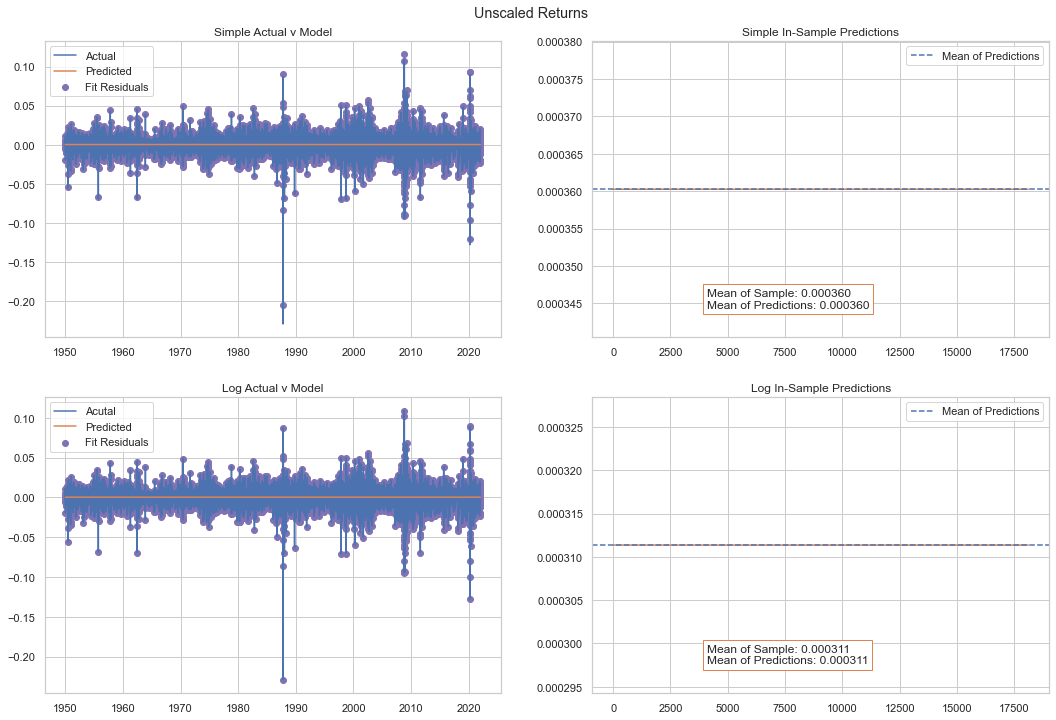
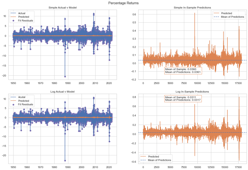
What we can see from the left-hand charts above is that the ARMA model is generally quite poor at predicting the daily fluctuations in share prices. The residuals are very large and the ARMAs account for only that very thin strip within the actual fluctations.
However, on the right-hand charts we can see that the ARMA processes account for essentially all of the time series mean.
GARCH Forecasting
We currently have a model describing the stationary and dependent mean process of our time-series. The resulting residuals should have a near-zero, constant mean.
But we can also see this model is very poor at describing daily returns. So now we look to incorporate volatility dependence via GARCH. This can be done by fitting a GARCH model to the residuals of the ARMA fit.
We will focus strictly on scaled simple returns.
[10]:
import pandas as pd

data = pd.Series(sparmasim100.resid(), index=sp_ret.index)
We use the arch_model class from the arch package, which defaults to GARCH(1,1).
[11]:
import arch

model = arch.arch_model(data, p=1, q=1)
model_fit = model.fit(disp='off')
model_fit.params.mu, sparmasim100.resid().mean()
[11]:
(0.01977812138048156, -6.663614539820898e-05)
This prodcues an interesting value in the mean. We expected a near-zero mean and ended up with a ~0.02%. By incorporating conditional volatility, we have essentially revealed a larger mean process within the residuals (or picked up an artifact therein).
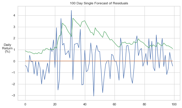
The model_fit object can be used to forecast future residual values.
[12]:
pred = model_fit.forecast(horizon=100, simulations=1, method='simulation', reindex=False)
We can see a single 100-day forecast below, resulting from the small, positive mean and the dynamic variance.
We can show how a forecast compares with actual data, by fitting against a past subset and projecting forward from the last fitted date.
[14]:
model = arch.arch_model(data[:-100], p=1, q=1)
model_fit = model.fit(disp='off')
GARCH models incorporate a stochastic error term generated from standard Gaussian white noise, so the value of any single simulation is minimal. Below we show the deviation of four forecasts relative to the actual.
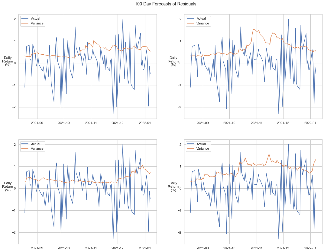
Projection with Expanding Window
We can arrive at a better fit to the data if we use a window-process. Time-series models can be fit either over the entire time-series or over a window. The intent is to capture any changes in the parameters of the series over time.
An expanding window approach fits the model on an ever-increasing window over a chosen increment. Below we show an expanding window incremented daily.
[16]:
from tqdm.auto import trange, tqdm

n = 100
vars_ = np.zeros(n)
means_ = np.zeros(n)
for i in trange(n):
    train = data[:-(n-i)]
    model = arch.arch_model(train, p=1, q=1)
    model_fit = model.fit(disp='off')
    pred = model_fit.forecast(horizon=1, reindex=False)
    means_[i] = pred.mean.values[-1][0]
    vars_[i] = np.sqrt(pred.variance.values[-1,:][0])
We can see below that the forecast variance fits very nicely with the actual. One should also note that the mean value changes slighlty over the 100-day forecast.
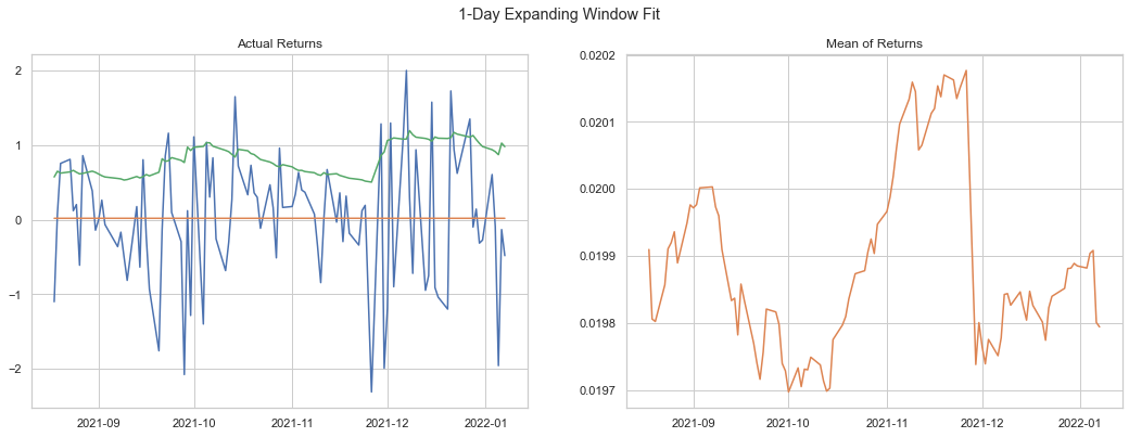
We can see this is especially true over a longer time period. Here we increase to 5,000 days.
[18]:
n = 5000
vars_ = np.zeros(n)
means_ = np.zeros(n)
for i in trange(n):
    train = data[:-(n-i)]
    model = arch.arch_model(train, p=1, q=1)
    model_fit = model.fit(disp='off')
    pred = model_fit.forecast(horizon=1, reindex=False)
    means_[i] = pred.mean.values[-1][0]
    vars_[i] = np.sqrt(pred.variance.values[-1,:][0])
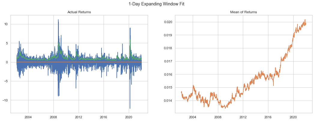
We can see the variance captures the spikes in daily changes very nicely. The mean does change but in a narrow range.
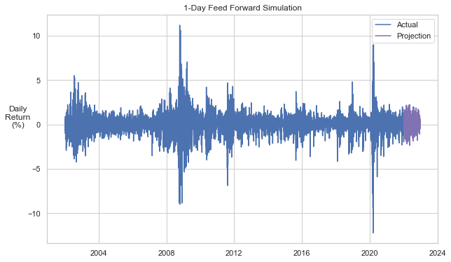
Feed Forward for Out-of-Sample Projections
Instead of using a multi-horizon forecast via the forecast method of arch, the forecast can be created by refitting a new model that incorporates the most recent forecast. We will show this process on just the last 20 years of data.
[20]:
n = 252
window = 5040
foredata = data[-window:].copy()
foredata = np.concatenate((foredata, np.zeros(n)*np.nan))
[21]:
values = np.zeros(n)
for i in trange(n):
    train = foredata[:-n+i]
    model = arch.arch_model(train, p=1, q=1)
    model_fit = model.fit(disp='off')
    pred = model_fit.forecast(horizon=1, simulations=1, method='simulation', reindex=False)
    values[i] = pred.simulations.values[0,0,0]
    foredata[-n+i] = values[i]
Below we can see the go-forward projection that results. Not a bad result, but it does seem like some of the more extreme values are not replicated.
Fixed Windows
Instead of an expanding window, a fixed window can be rolled forward. The observations may or may not overlap. This approach more directly captures state changes in the model that may occur over time, although it does also clip information.
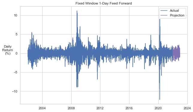
First, we show a fixed window on recent data (same as above) incremented forward daily for the last 252 days. This will utilize the same feed-forward forecast used above.
[98]:
import scipy.stats as scist

n = 252
window = 5040
foredata = data[-window:].copy()
foredata = np.concatenate((foredata, np.zeros(n)*np.nan))
[99]:
vars_ = np.zeros(n)
means_ = np.zeros(n)
errs_ = np.zeros(n)
for i in trange(n):
    model = arch.arch_model(foredata[i:-n+i], p=1, q=1)
    model_fit = model.fit(disp='off')
    pred = model_fit.forecast(horizon=1, reindex=False)
    means_[i] = pred.mean.values[-1][0]
    vars_[i] = np.sqrt(pred.variance.values[-1,:][0])
    errs_[i] = np.sqrt(vars_[i])*scist.norm.rvs()
    foredata[window + i] = means_[i] + errs_[i]
The result is below. Here we see perhaps a bit more variation. This may result from less smoothing through the smaller sample, different properties of the specific window, or it may be from the random error term.
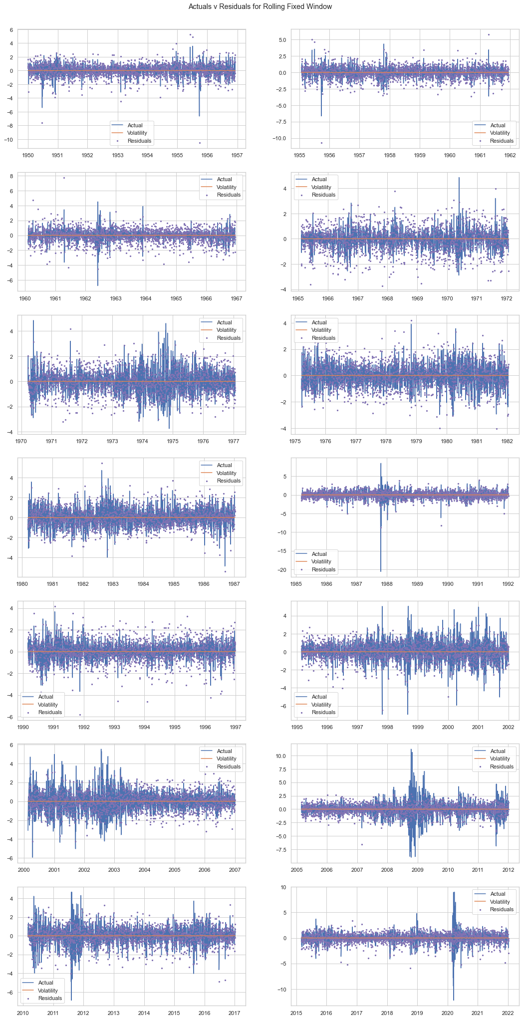
Fixed Window Across Entire Time Series
We will expand the above to fit a fixed window across the entire time series. We will drop two years of data with each shift in the window. This results in a window of ~13 years.
[26]:
n_windows = 13
drop = 252*5
window = data.size - n_windows*drop

windex = np.array([np.arange(drop*i+1, drop*i + window) for i in range(n_windows + 1)])
[27]:
vars_ = np.zeros((n_windows+1, window-1))
resids = np.zeros_like(vars_)
for i in trange(n_windows + 1):
    model = arch.arch_model(data[windex[i]], p=1, q=1)
    model_fit = model.fit(disp='off')
    resids[i] = model_fit.std_resid
Below we show the conditional volatility fit and the remaining residuals for each observation.
Garchcaster
Garchaster is a model for integrated ARMA-GARCH forecasting in phat.
Forecasting residuals is helpful but our goal is to develop a fulsome price simulation. To do that, we have to also incorporate the mean process in the ARMA model. In ARMA-GARCH both the mean and variance in the current period are functions of the residual in the prior period. So both ARMA and GARCH must be produced in conjunction at each step in the forecast.
The full ARMA-GARCH system looks as follows:
Note this does not exhaust the bevy of GARCH extensions: HARCH, FIGARCH, GJR-GARCH, etc.
The arch package has a forecast method built-in to its results object, however, we developed our own forecasting class to allow for some greater flexibility: Garchcaster. The class uses Numba to speed up processing time.
We will simulate 252 days of price movement 10,000 times.
Garchcaster requires the following inputs:
ARMA parameters
GARCH parameters
Standardized residuals from a GARCH fit
Conditional volaities from a GARCH fit
Residuals from a GARCH fit
Number of periods in the forecast
Number of iterations / simulations
[103]:
import phat as ph

days = 252
sims = 10000
mod = ph.Garchcaster(
    arma=sparmasim100.params()[:5],
    garch=model_fit.params.values,
    y=data.values.copy(),
    vols=model_fit.conditional_volatility.copy(),
    resids=model_fit.resid.copy(),
    iters=sims,
    periods=days,
)
rets = mod.forecast()
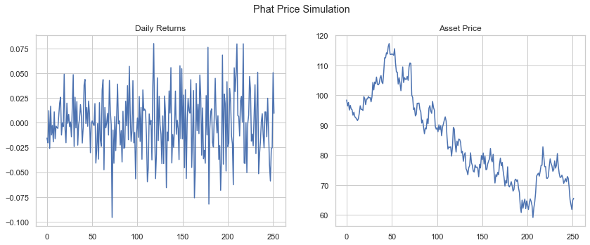
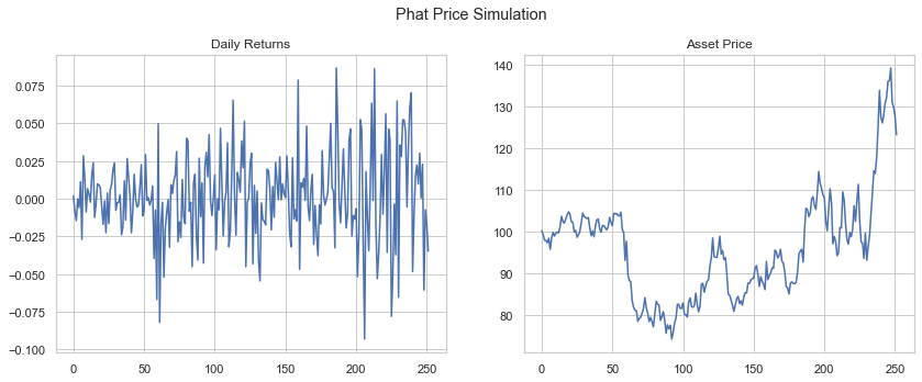
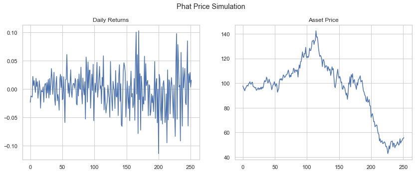
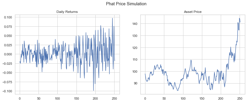
The GarchcastResults container has a number of chart devices available to inspect the data, including converting the daily returns into price. Below we show four sample iterations of the 252 day forecast, assuming the starting price of the asset was $100.
[104]:
rets.plot('price', p=100, n=4)
plt.show()
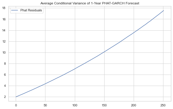
[106]:
plt.figure(figsize=(10,6))
plt.plot((rets.vols**2).T.mean(axis=1), label='Phat Residuals')
# plt.plot((res2.vols**2).T.mean(axis=1), label='N(0,1) Residuals')

plt.legend()
plt.title('Average Conditional Variance of 1-Year PHAT-GARCH Forecast')
plt.show()
We can show the distribution of prices on the final day of the forecast as well, while adding additional analysis on top.
[76]:
ax, S, bins = rets.plot('end_price', p=1)
plt.rcParams['patch.edgecolor'] = 'C0'

ax.axvline(S[:, -1].mean(), c='C1', ls='--', label=f'Mean: {S[:, -1].mean():.2f}')

logps = scist.lognorm.fit(S[:, -1])
x = np.linspace(0, 3.50, 1000)
lnormfit = scist.lognorm.pdf(x, *logps)
ax.plot(x, lnormfit, c='C2', label=r'$LogN$'+f'({logps[0]:.2f},{logps[1]:.2f},{logps[2]:.2f})')

ax.legend()
plt.show()
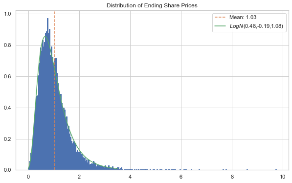
We can see that the body of the distribution is a strong fit for the lognormal, but the tail values are difficult to see. We can examine those better by comparing quantiles.
[77]:
l_crit = 1/np.logspace(2,5,4)
r_crit = 1 - l_crit
qs = np.concatenate((l_crit[::-1], r_crit))
logqs = scist.lognorm(*logps).ppf(qs)

actual = np.quantile(S[:,-1], qs)
pd.DataFrame(list(zip(logqs, actual)), index=qs, columns=['Lognorm', 'ARMA-GARCH'])
[77]:
| Lognorm | ARMA-GARCH | |
|---|---|---|
| 0.00001 | -0.057306 | 0.002942 |
| 0.00010 | -0.015758 | 0.007019 |
| 0.00100 | 0.047913 | 0.044852 |
| 0.01000 | 0.156496 | 0.133701 |
| 0.99000 | 3.149388 | 3.378547 |
| 0.99900 | 4.646870 | 5.960698 |
| 0.99990 | 6.370882 | 8.579409 |
| 0.99999 | 8.358290 | 9.625628 |
Interestingly, GARCH exhibits some modest fat-tailed behavior, even when using Gaussian error terms. This property has been understood since the very first GARCH paper by Bollerslev (1986).
Garchcaster Tests
As a check of the validity of the forecasts, we can compare to the same parameter setup from the arch forecast method. We’ll assume a constant mean process derived straight from the GARCH fit from arch.
First, we’ll show how the average variance at each day of the forecast compares by looking at small samples. We will generate just 20 samples, repeated 6 times.
Instead of passing all the required data separately, Garchcaster accepts arch and pmdarima results models directly. In this instance, we are using only a constant-mean garch resulting from the arch package.
[78]:
days = 252
sims = 20
mod = ph.Garchcaster(
    garch=model_fit,
    iters=sims,
    periods=days
)
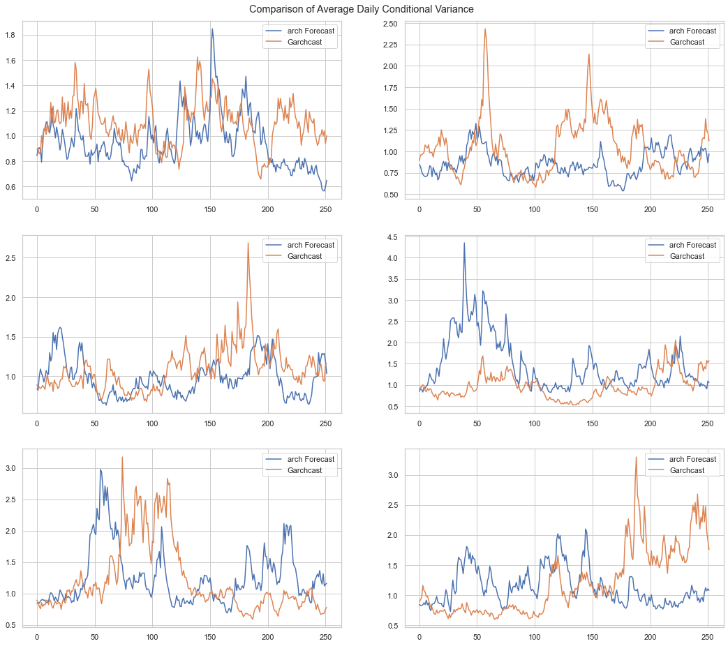
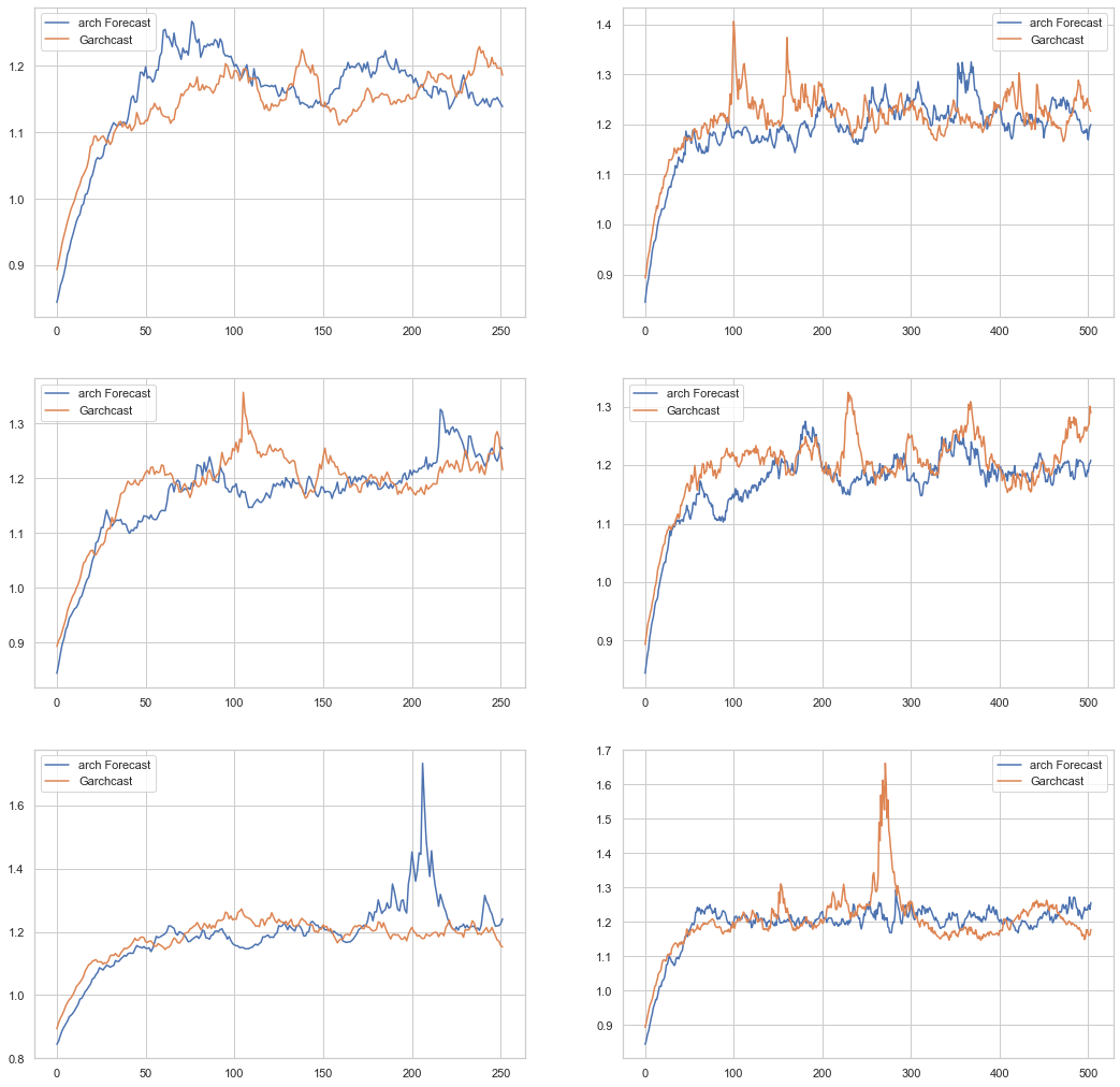
The two methods appear to create similar volatility behavior. If we increase the number of simulations, we can see that the methods tend towards the same stable value over time. The charts below show the average variance for 10,000 simulations over two time periods: 252 days and 504 days.
[80]:
days = 252
sims = 10000
mod = ph.Garchcaster(
    garch=model_fit,
    iters=sims,
    periods=days,
)
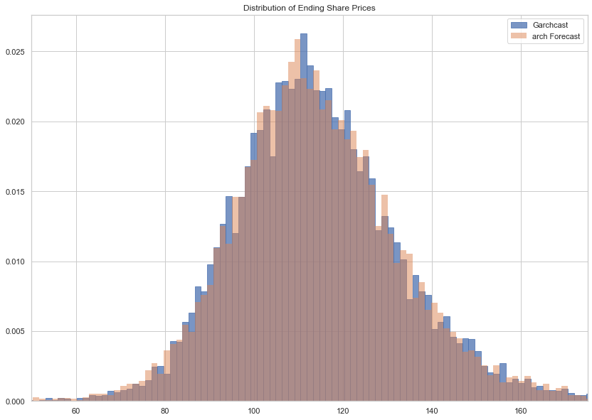
Below we see that the distribution of last period prices are almost identical for both methods.
[82]:
from phat.utils import PriceSim

fig, ax = plt.subplots(1,1, figsize=(14,10))

rets = mod.forecast(periods=252)
archsim = model_fit.forecast(horizon=252, simulations=sims, method='simulation', reindex=False)
ax, S, bins = rets.plot('end_price', p=100, ax=ax, label='Garchcast', alpha=.75)

simmer = PriceSim(100, periods=252, n=sims)
archsims_rets, archS, (ax, _) = simmer.sims(
    rets=archsim.simulations.values[0]/100+1,
    show_chart=True,
    ax=ax,
    bins=bins, lw=0, alpha=.5, label='arch Forecast'
)

ax.set_xlim(50, 175)

ax.legend()
plt.show()
As for speed:
[83]:
%timeit rets = mod.forecast(periods=252)
1.56 s ± 47.8 ms per loop (mean ± std. dev. of 7 runs, 1 loop each)
[84]:
%timeit archsim = model_fit.forecast(horizon=252, simulations=sims, method='simulation', reindex=False)
484 ms ± 7.61 ms per loop (mean ± std. dev. of 7 runs, 1 loop each)
We can see the custom forecast in phat-tails is about one-third as fast. Not great but also not bad given no parallelization and no other attempt to optimize has yet been employed.