Introduction
P.H.A.T. - Pareto Hybrids with Asymmetric Tails
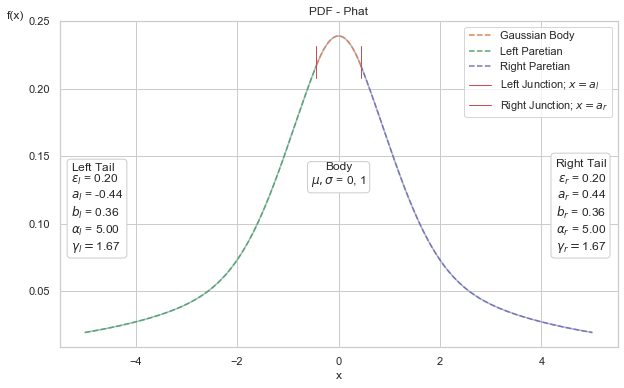
The Phat distribution is an attempt to address the issues of fat tails in two-tailed data. It is a two-tailed, fully-continuous, well-defined asymmetric power law probability distribution.
It is a mixture model of two Pareto hybrid distributions, as described in 2009 by Julie Carreau and Yoshua Bengio with:
Gaussian body
distinct Pareto power laws in either tail.
The distribution requires only 4 parameters:
\(\mu, \sigma\) in the Gaussian body
\(\xi_{\text{left}}, \xi_{\text{right}}\), being the inverse tail index (1/\(\alpha\)) for either Paretian tail.
The phat-tails package makes available several methods to fit a given time-series dataset to the parameters of the Phat distribution and produce a forecast with the results.
Quickstart
All pertinent classes and functions are imported via the module phat.
[130]:
import phat as ph
The probability distribution is found in the main class, Phat, which mimics the structure of the continuous distributions found in scipy.stats.
We pass the four parameters to instantiate the distribution. For simplicity, we will show the distribution with equal tail indices initially.
[131]:
mean, sig, shape = 0, 1, 1/5
phat_dist = ph.Phat(mean, sig, shape, shape)
Below is a complete rendering of the distribution, with breakdown among the component Gaussian and Pareto tails.
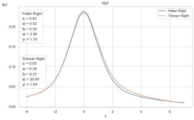
Below we demonstrate the ability to generate asymmetric tails. We overlay two different Phat distributions, one with symmetric tail indices of \(\alpha=2\) and the other with asymmetric tail indices, \(\alpha_{\text{left}}=2\) and \(\alpha_{\text{right}}=20\).
We can see that the left tails are identical. In the right tails, the distributions appear to differ only modestly, however, this difference leads to dramatically different effects.
[133]:
mean, sig = 0, 1
shape_l1, shape_r = 1/2, 1/2
dist1 = ph.Phat(mean, sig, shape_l1, shape_r)
shape_l2, shape_r = 1/2, 1/20
dist2 = ph.Phat(mean, sig, shape_l2, shape_r,)
The Phat class has common methods such as pdf, cdf, sf, ppf. It can also calculate negative log-likelihood and first and second moments. Derivations are found here.
[135]:
mean, sig, shape_l, shape_r = 0,1, 1/5, 1/4
phat_dist = ph.Phat(mean, sig, shape_l, shape_r)
phat_dist.pdf(10)
[135]:
array([0.00482994])
[136]:
phat_dist.cdf([.05,1,-0.1])
[136]:
array([0.51144212, 0.70624103, 0.47567736])
[137]:
phat_dist.sf([.05])
[137]:
array([0.48855788])
[138]:
assert phat_dist.sf([.05]) == 1 - phat_dist.cdf([.05])
[139]:
import numpy as np
phat_dist.ppf(np.linspace(0,1,5))
[139]:
array([ -inf, -1.63735173, 0.00569209, 1.68013031, inf])
[140]:
phat_dist.nll(1) # Negative Log-Likelihood
[140]:
array([1.8510368])
[141]:
phat_dist.mean()
[141]:
0.0796142959815449
[142]:
phat_dist.std()
[142]:
3.7926873955033087
It can also generate random variables (and standardized random variables).
[143]:
phat_dist.rvs(20)
[143]:
array([ 4.10522047,  3.55472489, -0.93678543,  0.51636282,  1.34579594,
        1.01540556, -0.80886831, -0.67534635,  0.09117024,  6.42834252,
        0.35292732,  3.1609973 ,  4.03059888,  5.0758071 , -3.4068779 ,
       -0.5631759 ,  0.76542791, -6.26470075, -5.32952901,  0.60021098])
[144]:
phat_dist.std_rvs(20)
[144]:
array([-0.12796173,  0.43906166, -0.737519  , -0.51000483,  0.17890436,
       -0.08411178,  0.28586079, -0.2721797 , -0.22500339,  0.22734977,
       -0.25146567,  0.64438798, -1.50587683,  0.1999281 , -0.29127155,
        0.35417953, -0.01986807,  0.5101493 ,  0.59852587, -0.38408617])
Importantly, Phat captures the undefined moments that result when \(\alpha < 2\).
[145]:
shape_l, shape_r, mean, sig = 1, 1, 0, 1
phat_dist = ph.Phat(mean, sig, shape_l, shape_r)
[146]:
phat_dist.mean()
/Users/spindicate/Documents/programming/investing/analysis/options/phat/src/phat/utils.py:75: RuntimeWarning: invalid value encountered in matmul
  return (self.p @ stack)
[146]:
nan
[147]:
phat_dist.var()
[147]:
nan
Phat has a fit method, which generates a standard Maximum Likelihood Estimate (MLE), although this is not the recommended approach to fitting this distribution.
In addition to the main distribution class, the package also provides:
ph.two_tailed_hill_double_bootstrap: a method for estimating both tail indices of a dataset simultaneouslyph.PhatNet: a simple neural network that provides improved fit relative to MLE, which includes a custom loss function calledPhatLoss.ph.Garchcaster: a class for generating time-series forecasts from ARMA and GARCH models that incorporates Phat random innovations.
Dependencies
Python versions: 3.9
numpy 1.19.5
numba 0.53.*
scipy 1.7.*
scikit-learn 0.24.*
statsmodels 0.12.*
tensorflow 2.5.0
tensorflow-probability 0.12.2
matplotlib 3.5.1
arch 4.19
pmdarima 1.8.2
tqdm 4.61.2
Also see requirements and compatibility specifications for Tensorflow and Numba
Suggested
tensorboard: monitoring tool for tensorflow
yfinance: for downloading historical price data
Also Check Out
-
built as part of Ivan Voitalov et al (2019) on tail index estimation techniques for power law phenomenon in scale-free networks
code from this package is utilized in the
two_tailed_hill_double_bootstrapfunction
thresholdmodeling for a package on manual Peak-over-Threshold (PoT) analysis.
Enhancements
Potential enhancements under consideration:
truncated Pareto tails
additional tail index estimation techniques
integration with Heston or other stochastic volatility models
incorporation of Phat innovations into
fitof AR-GARCH or ARMA-GARCH via custom modelgeneralization to additional GARCH models
better optimization of
Garchcaster.forecastmethod