Demo¶

Below we show a simple process for fitting and projecting a financial time series using phat. This example will utilize end-of-day daily prices of Coca-Cola, for which there is data back to 1962. The process is as follows:

download the daily prices of Coca-Cola (ticker: KO). Find the daily returns in percentage terms (i.e. x 100).
use the arch package to fit a GARCH(1,1) model to the daily returns
use the Hill double bootstrap method to estimate the tail index of both tails of the standardized residuals of the GARCH fit.
use phat custom data class, DataSplit, to split the data into training, testing, and validation subsets. Be careful to scale by 1/10.
use PhatNet and phat’s custom loss function PhatLoss to fit the remaining parameters.
use Garchcaster to produce 10,000 simulations of a one-year forecast via the same AR-GARCH model.

Download Data¶

[4]:

import yfinance as yf
import arch

import phat as ph

ko = yf.download('KO')
ko_ret = ko.Close.pct_change().dropna()*100
ko_ret = ko_ret[-252*10:]

[*********************100%***********************]  1 of 1 completed

Fit GARCH and Estimate \(\alpha\) in Both Tails¶

[5]:

res = arch.arch_model(ko_ret, mean='Constant', vol='Garch', p=1, q=1).fit(disp='off')
xi_left, xi_right = ph.two_tailed_hill_double_bootstrap(res.std_resid)

Fit \(\mu\) and \(\sigma\) with Machine Learning¶

[7]:

data = ph.DataSplit(res.std_resid[2:]/10)
pnet = ph.PhatNet(neurons=1)
pnet.compile(
    loss = ph.PhatLoss(xi_left,xi_right),
    optimizer = 'adam'
)
history = pnet.fit(data.train, validation_data=data.test, epochs=100, verbose=0)

Epoch 00046: early stopping

The training process above results in the following estimated parameters for the standardized GARCH residuals.

[8]:

pnet.predicted_params()

[8]:


mean	0.009800
sig	0.034620
shape_l	0.346772
shape_r	0.285840

Compare Fit with Gaussian and T¶

Below we compare the fit of the Phat distribution to that of the Gaussian and the Student’s T. Note the Student’s T fits to \(v=4.65\), which is equivalent to \(\xi = 0.22\), which is a thinner tail than found through the Hill Double bootstrap, particularly for the left tail.

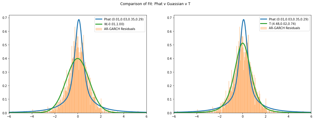
The Phat distribution is a better fit to the peak of the distribution while both the Gaussian and Student’s T are better fits in the shoulders. The devil, of course, is in the tails.

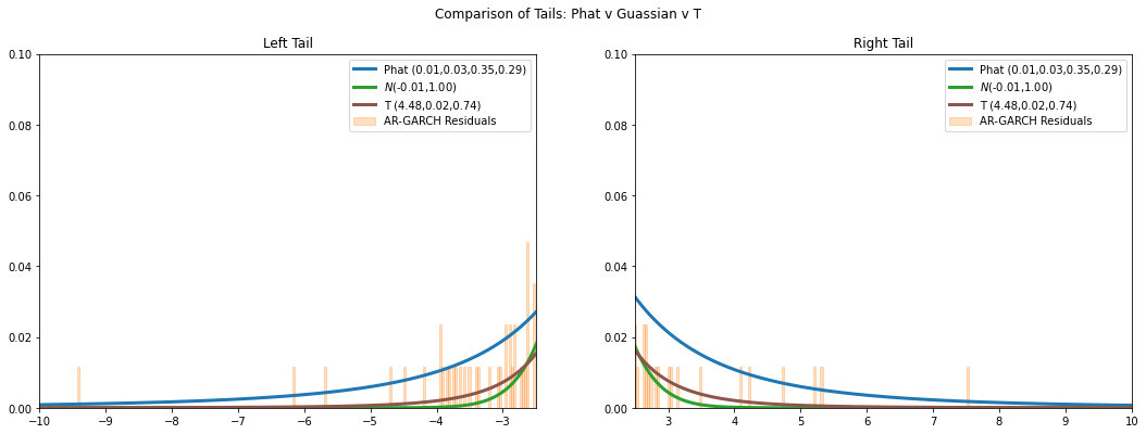
Out in the left and right tails we see the Phat distribution is much better at capturing extreme events that have occured in the past 10 years.

Generate Garch Forecasts¶

We can then feed this distribution, along with the results from the AR-GARCH fit, into the Garchcaster.

[15]:

n = 10000
days = 252

mu, sig, l, r = pnet.predicted_params().values
phatdist = ph.Phat(mu*10, sig*10, l, r)
fore = ph.Garchcaster(
    garch=res,
    iters=n,
    periods=days,
    order=(0,0,1,1),
    dist=phatdist
).forecast()

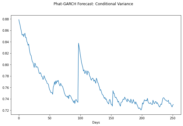
Calling the forecast method results in 10,000 separate AR-GARCH simulations, each spanning 252 trading days. A GarchcastResults container is returned, which includes some plotting methods for convenience.

We can see the conditional variance of the resulting forecasts.

[16]:

fore.plot('var')
plt.show()

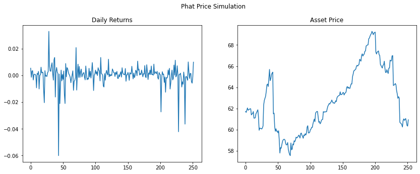
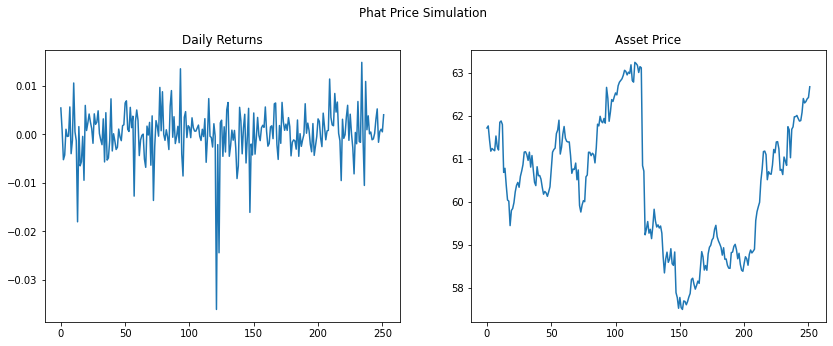
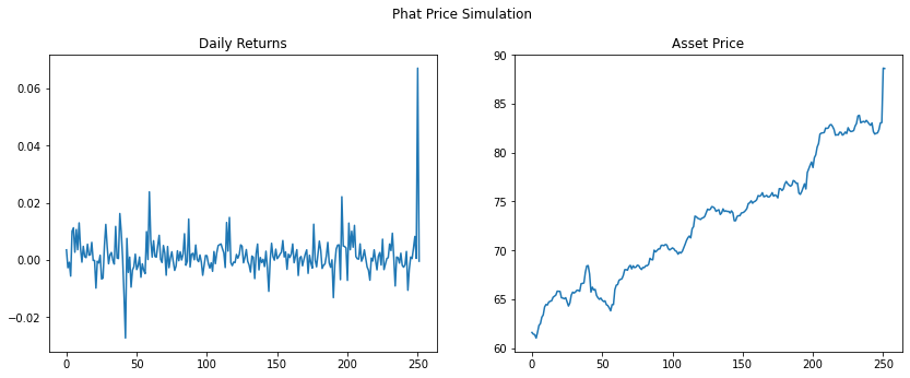
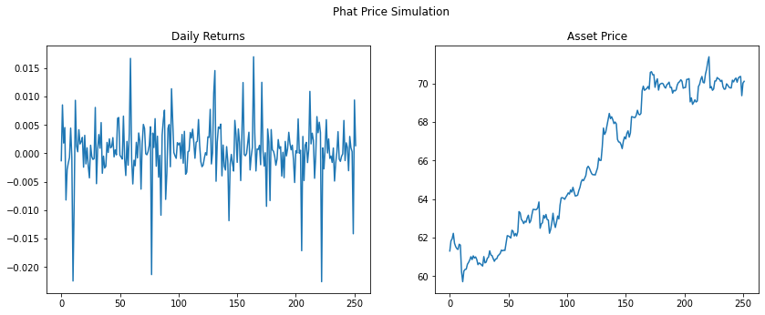
We can plot individual simulations.

[17]:

fore.plot('price', p=ko.Close[-1], n=4)
plt.show()

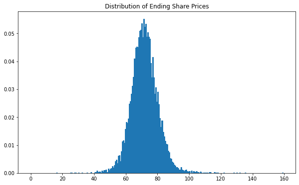
And we can plot a histogram of the final price in each simulation.

[18]:

ax, P, bins = fore.plot('end_price', p=ko.Close[-1], ec='C0')
plt.show()

phat-tails 0.0.11 documentation