Introduction
The Phat distribution is a two-tailed, fully-continuous, well-defined asymmetric power law probability distribution.
The phat package makes available several methods to fit a given time-series dataset to the parameters of the Phat distribution and produce a forecast with the results.
Installation
Installation available via pip
$ pip install phat-tails
Dependencies
Python versions: 3.9
numpy 1.19.5
numba 0.53.*
scipy 1.7.*
scikit-learn 0.24.*
statsmodels 0.12.*
tensorflow 2.5.0
tensorflow-probability 0.12.2
matplotlib 3.5.1
arch 4.19
pmdarima 1.8.2
tqdm 4.61.2
Also see requirements and compatibility specifications for Tensorflow and Numba
Suggested
tensorboard: monitoring tool for tensorflow
yfinance: for downloading historical price data
Also Check Out
-
built as part of Ivan Voitalov et al (2019) on tail index estimation techniques for power law phenomenon in scale-free networks
code from this package is utilized in the
two_tailed_hill_double_bootstrapfunction
thresholdmodeling for a package on manual Peak-over-Threshold (PoT) analysis.
Enhancements
Potential enhancements under consideration:
truncated Pareto tails
additional tail index estimation techniques
integration with Heston or other stochastic volatility models
incorporation of Phat innovations into
fitof AR-GARCH or ARMA-GARCH via custom modelgeneralization to additional GARCH models
better optimization of
Garchcaster.forecastmethodsimplify
Garchcasterinterface
The Issue with Fat Tails
Many phenomena are understood to exhibit fat tails: insurance losses, wealth distribution, rainfall, etc. These are one-tailed phenomenom (usually bounded by zero) for which many potential distributions are applicable: Weibull, Levy, Frechet, Paretos I-IV, the generalized Pareto, the Extreme Value distribution etc.
Unfortunately, for two-tailed phenomenon like financial asset returns, there are only two imperfect candidates:
Levy-Stable Distribution
the Levy-Stable is bounded in the range \(\alpha \in (0, 2]\) with \(\alpha = 2\) being the Gaussian distribution. Thus, the Levy-Stable only exhibits fat tails with tail index \(\alpha < 2\)
Unfortunately, equity returns in particular are known to have both a second moment AND fat tails (see Danielsson and de Vries 1997), meaning \(\alpha > 2\), which the Levy-Stable does not support.
Student’s T
the Student’s T is the most popular distribution for modelling asset returns as it does exhibit modest fat tails and is power law-like.
unfortunately, the Student’s T only tends toward a power law in the extreme tails and so can still heavily underestimate extreme events.
also, the Student’s T is symmetric and cannot accomodate different tail indices in either tail. Nor can the skewed Student’s T, which is asymmetric, but accepts only a single tail index (although recently an asymmetric Student’s T has been proposed).
the Phat Distribution
The Phat distribution is an attempt to address the issues of fat-tails in two-tailed data. It is a mixture model of two Pareto hybrid distributions, as described in 2009 by Julie Carreau and Yoshua Bengio (and dubbed by us as the “Carben” distribution). The Carben is a piece-wise combination of a single Gaussian distribution and a generalized Pareto distribution fused at the Pareto location, \(a\).
The result is a distribution with Gaussian-body and distinct Pareto power laws in either tail. The distribution requires only 4 parameters:
\(\mu, \sigma\) in the Gaussian body
\(\xi_{\text{left}}, \xi_{\text{right}}\), being the inverse tail index for either Paretian tail.
Below, we show a Phat distribution with a standard normal body and symmetric Paretian tails with \(\xi = .2\) (corresponding to \(\alpha = 5\)), highlighting the distributions different sections.

The Paretian tails are parameterized independently and so allow for asymmetry. Below we show two Phat distributions, one with symmetric tail index of \(\alpha=2\) and the other with asymmetric tail indices, \(\alpha_{\text{left}}=2\) and \(\alpha_{\text{right}}=20\).
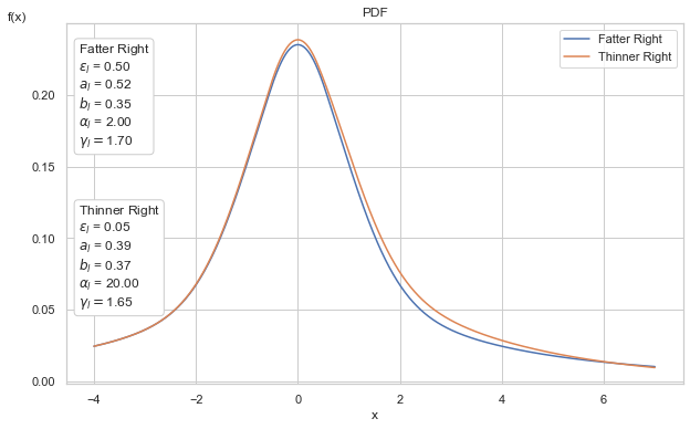
The left tails are identical. In the right tails, the distribution with the greater tail index has a slightly lower probability in the body and a slightly higher probability out in the tails, leading to dramatically different effects.